Reading and writing from disk
In the Getting started tutorial, we showed how rhodent is able to read a time-dependent wave functions file, construct density matrices in the Kohn-Sham basis, and take (inverse) Fourier transforms before calculating observables. Performing these transformations in memory is the fastest way to obtain observables. However, it has the disadvantage of being very memory intensive, in particular in parallel execution.
Here, we demonstrate how to write the density matrices to disk after transformation, and how to read them again in order to calculate observables. Splitting up the calculation in these two parts reduces the memory footprint, as different kinds of are held in memory for the different calculations.
We need the following files, that are obtained by following the steps in Preparations.
ksd.ulm- KohnShamDecomposition file.wfs.ulm- Time-dependent wave functions file after excitation by the sinc-shaped pulse.
Write to disk in the frequency domain
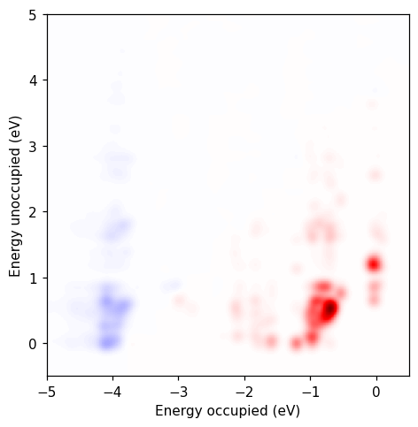
In the Getting started tutorial we calculated the transition contribution map (TCM) for the absorption spectrum. Here, we perform the same calculation in two steps.
First, we set up a ResponseFromWaveFunctions with the wfs.ulm and ksd.ulm files, additionally specifying the perturbation used in the TDDFT calculation. Then, we call the write_in_frequency function to calculate the (normalized) response in the frequency domain and write to disk.
We specify a format string which tells rhodent how to name the resulting files. The format string supports the variables
freqandreim.We want to compute the response at 3.8eV with 0.1eV Gaussian broadening.
We only calculate the Fourier transform of the real part of the density matrix, but not of the imaginary part, as we won’t need the latter.
The Fourier transform of the density matrix will now be computed from the time-dependent wave functions file wfs.ulm, normalized by the perturbation, and written to disk. In this case, we only write the one file frho_broadened/w03.80-Re.npy.
[ ]:
from rhodent.response import ResponseFromWaveFunctions

# Set up the perturbation used in the TDDFT calculation
perturbation = {'name': 'SincPulse',
                'strength': 1e-6,  # Amplitude
                'cutoff_freq': 8,  # Cut-off frequency in units of eV
                'time0': 5,  # Time of maximum in number of oscillations
                'relative_t0': True}

# Set up a response from the time-dependent wave functions file
response = ResponseFromWaveFunctions(wfs_fname='wfs.ulm',
                                     ksd='ksd.ulm',
                                     perturbation=perturbation)

# Write the Fourier transform of the density matrix to disk
response.write_in_frequency('frho_broadened/w{freq:05.2f}-{reim}.npy',
                            frequencies=[3.8],
                            frequency_broadening=0.1,
                            real=True,
                            imag=False)
Now we perform a separate calculation to calculate the TCM. We set up a ResponseFromFourierTransform with the ksd.ulm file and the same format string. Then we set up the DipoleCalculator and calculate the TCM. We get the same results as if we had done the entire calculation in one go.
Warning
Because we specified the perturbation in the previous step, the response written to disk is already normalized. We do not specify the perturbation again, as this would divide by the Fourier transform of the perturbation once again.
[ ]:
import numpy as np
from rhodent.response import ResponseFromFourierTransform
from rhodent.calculators import DipoleCalculator

# Set up the response from disk
response = ResponseFromFourierTransform('frho_broadened/w{freq:05.2f}-{reim}.npy',
                                        ksd='ksd.ulm')

# Set up the dipole calculator. We do not specify the frequency_broadening argument,
# as the density matrices on disk are already broadened
calc = DipoleCalculator(response=response,
                        energies_occ=np.arange(-5, 1.001, 0.01),
                        energies_unocc=np.arange(-1, 5.001, 0.01),
                        sigma=0.07,
                        frequencies=[3.8])

# Calculate the dipole contributions
calc.calculate_and_write('tcm.npz', include_tcm=True)
                ###     #####
               ###############
         ########  #####     ##
     ###########            ###           _               _            _
  #######                  ###       _ __| |__   ___   __| | ___ _ __ | |_
 ####                      ##       | '__| '_ \ / _ \ / _` |/ _ \ '_ \| __|
 #                          ##      | |  | | | | (_) | (_| |  __/ | | | |_
 #                           ##     |_|  |_| |_|\___/ \__,_|\___|_| |_|\__|  0.1
 #                            ##
 #                             ##
 ##                             ###
  ####                           ###
   ##########                     ##
      ########                   ###
            ###                ####
            ##               ####
            ##           ######
            #################

Date:   Tue Jun 10 10:39:30 2025
CWD:    /cfs/klemming/projects/supr/plasmons/fojt/rhodent-supplementary/notebooks/restarting
cores:  1
Python: 3.12.0
numpy:  /cfs/klemming/projects/supr/cms/fojt/conda-gpaw-frozen/lib/python3.12/site-packages/numpy (version 1.26.0)
ASE:    /cfs/klemming/home/f/fojt/.local/lib/python3.12/site-packages/ase (version 3.25.0)
GPAW:   /cfs/klemming/home/f/fojt/git/gpaw/frozen/gpaw (version 25.1.0)

[00:00:00.0] Set up calculator:
================  DipoleCalculator  =================
response:
  ResponseFromFourierTransform
    ksd: ksd.ulm
    frho_fmt: frho_broadened/w{freq:05.2f}-{reim}.npy
    perturbation:
      No perturbation

voronoi:
  No Voronoi decomposition

Energies for broadening (sigma = 0.1 eV)
  Occupied: 601 from -5.0 to 1.0 eV
  Unoccupied: 601 from -1.0 to 5.0 eV
-----------------------------------------------------

==================================
 Procedure for obtaining response
==================================
Response from Fourier transform of density matrices on disk

Format string: frho_broadened/w{freq:05.2f}-{reim}.npy
Calculating response for 1 frequencies
  frequencies: 3.8 eV

=================
 Memory estimate
=================
Reading response:
    Unknown

........................
.. Total on all ranks ..
........0.0 MiB.........

[00:00:13.1] [Calculator] Calculated and broadened dipoles contributions in 1.24s for Re @ Freq. 3.800eV
[00:00:13.1] [Calculator] Finished calculating dipoles contributions
[00:00:13.2] [Calculator] Written tcm.npz
[ ]:
import numpy as np
from matplotlib import pyplot as plt
from matplotlib.colors import Normalize

# Load the transition contribution map
archive = np.load('tcm.npz')

osc_ou = archive['dm_wouv'][0, :, :, 2].imag * archive['osc_prefactor_w'][0]
energy_o = archive['energy_o']
energy_u = archive['energy_u']

# Setup axis
fig, ax = plt.subplots(1, 1, figsize=(6, 4.5))

vmax = np.max(np.abs(osc_ou))
norm = Normalize(-vmax, vmax)

# Plot the transition contribution map
ax.pcolormesh(energy_o, energy_u, osc_ou.T, cmap='seismic', norm=norm)

ax.set_aspect('equal',adjustable='box')
ax.set_xlim([-5, 0.5])
ax.set_ylim([-0.5, 5])

ax.set_xlabel('Energy occupied (eV)')
ax.set_ylabel('Energy unoccupied (eV)')

fig.tight_layout()
Write to disk after pulse convolution
Now, we will split up the calculation of the time-evolution of stored energy. Similar to the previous example, we could use the write_in_time function of the response object to perform the pulse convolution and then write the density matrices to disk. One inconvenient detail, however, is that we need to specify which derivatives (in the time domain) of the density matrix to compute, or whether to compute real and/or imaginary parts (in the frequency domain). We can circumvent this by setting
up the calculator and using the write_response_to_disk function, which is just a wrapper for write_in_time or write_in_frequency that ensures that the necessary density matrices are written.
We set up the ResponseFromWaveFunctions and EnergyCalculator in the same way is if we were to do the calculation in one go. Then, we call write_response_to_disk with a format string specifying the file names. The format string supports the variables pulsefreq, pulsefwhm, time and tag. The pulse convolution is
performed, and density matrices are written to disk. Because the EnergyCalculator needs density matrices (for example pulserho_pf3.80/t0029920.0.npy) and their first derivatives (for example pulserho_pf3.80/t0029920.0-Iomega.npy), both are written.
[ ]:
import numpy as np
from rhodent.calculators import EnergyCalculator
from rhodent.response import ResponseFromWaveFunctions

# Set up the perturbation used in the TDDFT calculation
perturbation = {'name': 'SincPulse',
                'strength': 1e-6,  # Amplitude
                'cutoff_freq': 8,  # Cut-off frequency in units of eV
                'time0': 5,  # Time of maximum in number of oscillations
                'relative_t0': True}

# Set up a response from the time-dependent wave functions file
response = ResponseFromWaveFunctions(wfs_fname='wfs.ulm',
                                     ksd='ksd.ulm',
                                     perturbation=perturbation)

# Set up a calculator for a list of times and pulses
pulses = [{'name': 'GaussianPulse',
           'strength': 1e-6, # Amplitude
           'frequency': pf,  # Frequency in units of eV
           'time0': 10e3,  # Time of maximum in units of fs
           'sigma': 0.3,  # Parameter related to width in frequency domain, in units of eV
           'sincos': 'cos'} for pf in [3.3, 3.8]]
calc = EnergyCalculator(response,
                        times=np.linspace(0, 30e3, 300),
                        pulses=pulses)

# Perform the pulse convolution, then write the density matrices
# and all necessary derivatives to disk
calc.write_response_to_disk('pulserho_pf{pulsefreq:.2f}/t{time:09.1f}{tag}.npy')
For the second calculation, we set up a ResponseFromDensityMatrices with the same format string. Since we want the response to two different pulses, we have to supply them again. Because the format string contains the pulsefreq variable, rhodent will read the right files for each pulse. Importantly, we do not specify the perturbation, as rhodent would then try to perform pulse convolution on the already
convoluted data.
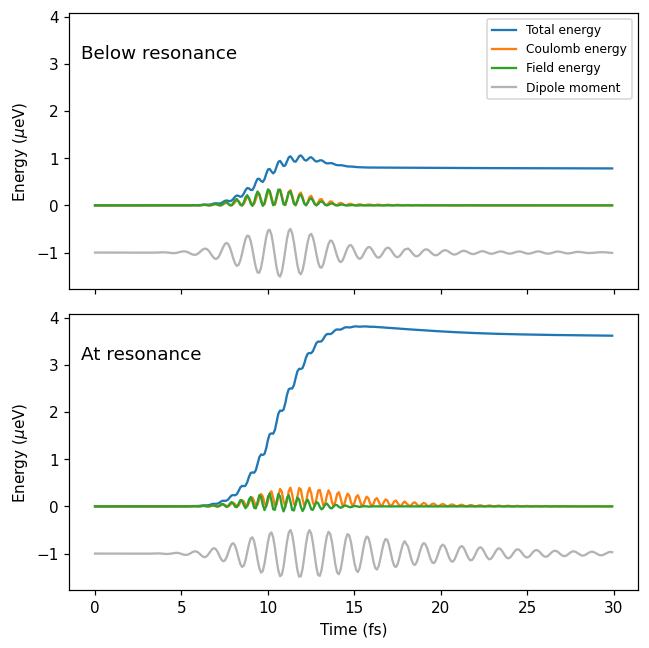
We set up an EnergyCalculator and calculate the time-evolution of the energies. Plotting the energies, we see that the results are the same as when we did the calculation in one go in the Getting started tutorial.
Note
The ResponseFromFourierTransform looks for all files on disk that match the format string, before choosing which ones to use. In this example, files t0000010.0.npy, t0000110.0.npy, t0000210.0.npy are written to disk, as they correspond to times written in the TDDFT calculation. When we ask rhodent to read times np.linspace(0, 30e3, 300), it chooses the nearest available times.
[ ]:
import numpy as np
from rhodent.perturbation import create_perturbation
from rhodent.response import ResponseFromDensityMatrices
from rhodent.calculators import EnergyCalculator

pulses = [{'name': 'GaussianPulse',
           'strength': 1e-6, # Amplitude
           'frequency': pf,  # Frequency in units of eV
           'time0': 10e3,  # Time of maximum in units of fs
           'sigma': 0.3,  # Parameter related to width in frequency domain, in units of eV
           'sincos': 'cos'} for pf in [3.3, 3.8]]

# Set up a response without a perturbation specified
response = ResponseFromDensityMatrices(
        pulserho_fmt='pulserho_pf{pulsefreq:.2f}/t{time:09.1f}{tag}.npy',
        ksd='ksd.ulm')
calc = EnergyCalculator(response,
                        times=np.linspace(0, 30e3, 300),
                        pulses=pulses)

# Calculate the energies
calc.calculate_and_write('energy.npz', only_one_pulse=False)
[ ]:
import numpy as np
from matplotlib import pyplot as plt

archive = np.load('energy.npz')

fig, axes = plt.subplots(2, 1, figsize=(6, 6), sharex=True, sharey=True)
for p, ax in enumerate(axes):
    ax.plot(archive['time_t'], 1e6 * archive['total_pt'][p], label='Total energy')
    ax.plot(archive['time_t'], 1e6 * archive['total_Hxc_pt'][p], label='Coulomb energy')
    ax.plot(archive['time_t'], 1e6 * archive['Epulse_pt'][p], label='Field energy')
    dm_t = archive['dm_pt'][p]
    ax.plot(archive['time_t'], -1 + 0.5 * dm_t / dm_t.max(), color='0.7', label='Dipole moment')
ax.set_xlabel('Time (fs)')
axes[0].set_ylabel(r'Energy ($\mu$eV)')
axes[1].set_ylabel(r'Energy ($\mu$eV)')
axes[0].set_title('Below resonance', x=0.02, y=0.85, va='top', ha='left')
axes[1].set_title('At resonance', x=0.02, y=0.85, va='top', ha='left')
axes[0].legend(fontsize=8)

fig.tight_layout()