The convolution trick

The purpose of this page is to show that responses to arbitrary pulses are related to each other, as long as the response is in the linear regime, and the pulses overlap in frequency. We can take advantage of this relation by performing one expensive TDDFT calculation with a pulse that has a broad spectral response (like a delta-kick or sinc-shaped pulse), and in post-processing obtain the response to any other pulse.

To perform the exercises, we need the following files, that are obtained by following the steps in Preparations.

• ksd.ulm - KohnShamDecomposition file

• wfs.ulm - Time-dependent wave functions file after excitation by sinc-shaped pulse

• dm.dat - Dipole moment file after excitation by sinc-shaped pulse

• wfs_delta.ulm - Time-dependent wave functions file after excitation by delta-kick

• dm_delta.dat - Dipole moment file after excitation by delta-kick

• wfs_gauss.ulm - Time-dependent wave functions file after excitation by Gaussian pulse

• dm_gauss.dat - Dipole moment file after excitation by Gaussian pulse

We will also need the following files from the Getting started tutorial.

• voronoi.ulm - File with Voronoi weights

• hcdist_proj.dat - Data file with projected hot-carrier distributions

Plotting the perturbations

Let plot the three different perturbations used in the TDDFT calculations, in the time and frequency domains. We set up Perturbation objects for this purpose.

• The amplitude method returns the perturbation in the time domain, for a grid of times in atomic units.

• The frequencies method returns a grid of frequencies in atomic units. As arguments, it takes a grid of times, and a data length. By supplying a length that is longer than the time grid, the frequencies grid is made more dense.

• The fourier method returns the Fourier transform of the perturbation, given a grid of times and data length.

Internally, these objects use the fft module of numpy to take the Fourier transform. By working with real data in the time domain, only the positive frequency axis of the Fourier transform is needed.

When plotting, we convert from atomic units of time to femtoseconds and atomic units of frequency to electron volts by multiplying the grids with the conversion factors au_to_fs and au_to_eV.

import numpy as np
from matplotlib import pyplot as plt
from gpaw.tddft.units import au_to_fs, au_to_eV

# Set up a dense time grid in atomic units
times = np.linspace(0, 1200, 500)
timestep = times[1] - times[0]

# Specify a number of data samples that is longer than our data,
# causing our data to be zero padded before Fourier transformation.
# For now, this is for visualization purposes only, but later we
# will do this to break the periodicity of the Fourier transform.
padnt = 2 * len(times)  # Number of times, including zero padding


def plot(perturbation, exp):
    fig, axes = plt.subplots(1, 2, figsize=(6, 2.4))

    # Pulse in the time domain
    pulse_amplitudes = perturbation.amplitude(times)
    scale = 10**(-exp)
    axes[0].plot(times * au_to_fs, scale * pulse_amplitudes)
    axes[0].set(xlabel='Time (fs)', ylabel=fr'Amplitude $\times 10^{{{exp}}}$')

    # Pulse in the frequency domain
    frequencies = perturbation_sinc.frequencies(times, padnt)
    pulse_fourier = perturbation.fourier(times, padnt)
    axes[1].plot(frequencies * au_to_eV, scale * pulse_fourier.real, label='Re')
    axes[1].plot(frequencies * au_to_eV, scale * pulse_fourier.imag, label='Im')
    axes[1].plot(frequencies * au_to_eV, scale * np.abs(pulse_fourier), label='Abs',
                 color='k', lw=1)
    axes[1].set(xlabel='Frequency (eV)', xlim=[0, 10])

    fig.tight_layout()

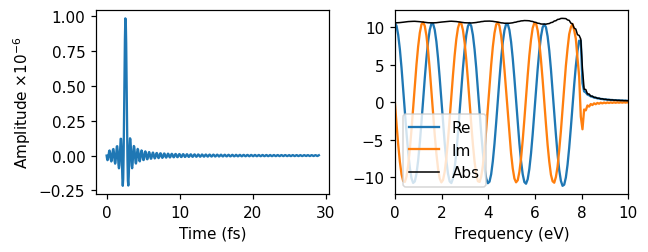
Sinc-shaped pulse

First, we ran real-time TDDFT with a sinc-shaped pulse. The parameters are chosen such that the amplitude, in the time domain, is close to zero in the beginning of the simulation. The maximum amplitude occurs after 5 oscillations. In the frequency domain, the absolute value of the pulse is relatively constant up to 8 eV, where it is smoothly cut off. By perturbing the system with this pulse, we are thus exciting up to 8 eV frequency-components of the response.

from rhodent.perturbation import create_perturbation

# Set up perturbations
perturbation_sinc = create_perturbation(
        {'name': 'SincPulse',
         'strength': 1e-6,  # Amplitude
         'cutoff_freq': 8,  # Cut-off frequency in units of eV
         'time0': 5,  # Time of maximum in number of oscillations
         'relative_t0': True})

print(perturbation_sinc)
plot(perturbation_sinc, -6)
plt.legend(loc='lower left');

name: SincPulse, strength: 1e-06, time0: 5
cutoff_freq: 8, relative_t0: True

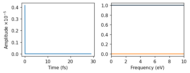
Delta-kick

Then, we used a delta-kick, which is a perturbation that is exacly constant (and real) in frequency space. The strength of the delta kick is specified in the frequency domain to ${10}^{-5}$.

perturbation_delta = create_perturbation(
        {'name': 'deltakick',
         'strength': 1e-5,  # Strength in frequency domain
        })

print(perturbation_delta)
plot(perturbation_delta, -5)

Delta-kick perturbation (strength 1.0e-05)

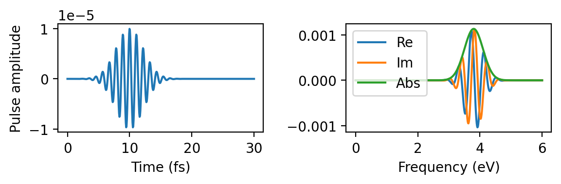
Gaussian pulse

Finally, we used a Gaussian pulse pulse of frequency 3.8 eV with a maximum in the time domain at 10 fs. The sigma parameter (0.3 eV) corresponds to a full width at half-maximum (FWHM) of about 0.7 eV in the frequency domain and 5 fs in the time domain.

perturbation_gauss = create_perturbation(
        {'name': 'GaussianPulse',
         'strength': 1e-6, # Amplitude
         'frequency': 3.8,  # Frequency in units of eV
         'time0': 10e3,  # Time of maximum in units of fs
         'sigma': 0.3,  # Parameter related to width in frequency domain, in units of eV
         'sincos': 'cos'})

print(perturbation_gauss)
plot(perturbation_gauss, -5)

name: GaussianPulse, strength: 1e-06
time0: 10000.0, frequency: 3.8, sigma: 0.3
sincos: cos

Performing the pulse convolution

Now, we will demonstrate how the response to one perturbation can be obtained from the response to another perturbation. As an instructive example, we begin with the dipole moment.

In the linear response regime, we can express the dipole moment $\mathit{d}$ as the polarizability times the external perturbation in the (spatially constant) electric field. In the frequency domain

$$\mathit{d}(\omega )=\mathit{\alpha }(\omega ){\mathit{E}}_{\text{ext}}(\omega ),$$

or, equivalently, in the time domain

$$\mathit{d}(t)={\int }_0^t\mathit{\alpha }(t-t^{\prime }){\mathit{E}}_{\text{ext}}(t^{\prime })\mathrm{d}{t}^{\prime }.$$

Therefore, if we know the dipole response to one perturbation (e.g. ${\mathit{d}}_{\mathrm{sinc}}$ to a sinc perturbation ${\mathit{E}}_{\text{sinc}}$), then we know the polarizability (at least at frequencies where the perturbation is non-zero). Hence, we can reconstruct the response to any other perturbation (e.g. ${\mathit{d}}_{\mathrm{gauss}}$ to a Gaussian laser field ${\mathit{E}}_{\text{gauss}}$). This is most easily obtained in frequency space

$$\begin{array}{r}\begin{array}{rl}{\mathit{d}}_{\text{gauss}}(\omega )& =\mathit{\alpha }(\omega ){\mathit{E}}_{\text{gauss}}(\omega )\\ & =\frac{{\mathit{d}}_{\text{sinc}}(\omega )}{{\mathit{E}}_{\text{sinc}}(\omega )}{\mathit{E}}_{\text{gauss}}(\omega ).\end{array}\end{array}$$

The polarizability is a 3x3 tensor and its full calculation requires three separate TDDFT calculations with perturbations in different directions. For simplicity, we will assume that the perturbations of interest for us are in the same direction, and we can thus use the scalar amplitudes $v(\omega )$ of the perturbations.

$$\begin{array}{rl}{\mathit{d}}_{\text{gauss}}(\omega )& ={\mathit{d}}_{\text{sinc}}(\omega )\frac{v_{\text{gauss}}(\omega )}{v_{\text{sinc}}(\omega )}.\end{array}$$

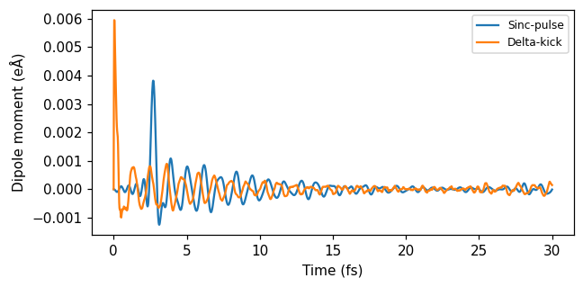
Read and plot the dipole moment

First, we read the dipole moment files dm.dat, dm_delta.dat containing ${\mathit{d}}_{\text{sinc}}(t)$, and ${\mathit{d}}_{\text{delta}}(t)$.

from gpaw.tddft.units import au_to_eA


def read_dipole_file(filename):
    """ Read dipole moment file.

    Return the time (in atomic units) and the
    z-component of the dipole moment (in units of eÅ).

    Discard step-like data, and repeated data due to restarts.
    Subtract the static dipole.
    """
    # Read dipole moment file and subtract static dipole
    time_t, _, _, _, dm_t = np.loadtxt(filename, unpack=True)
    dm_t -= dm_t[0]
    dm_t *= au_to_eA  # Convert from atomic units to eÅ

    # Remove any non-increasing times (due to restart of kick)
    flt_t = np.ones_like(time_t, dtype=bool)
    maxtime = time_t[0]
    for t in range(1, len(time_t)):
        if time_t[t] > maxtime:
            maxtime = time_t[t]
        else:
            flt_t[t] = False
    time_t = time_t[flt_t]
    dm_t = dm_t[flt_t]
    return time_t, dm_t


# Read times and dipole moments in atomic units
times_sinc, dipole_moments_sinc = read_dipole_file('dm.dat')  # After sinc-pulse
times_delta, dipole_moments_delta = read_dipole_file('dm_delta.dat')  # After delta-kick

# Plot
fig, ax = plt.subplots(1, 1, figsize=(6, 3))

ax.plot(times_sinc * au_to_fs, dipole_moments_sinc, label='Sinc-pulse')
ax.plot(times_delta * au_to_fs, dipole_moments_delta, label='Delta-kick')

ax.set(xlabel='Time (fs)', ylabel=r'Dipole moment (eÅ)')
ax.legend(loc='upper right', fontsize=8)

fig.tight_layout()

Then, we compute the polarizability from the sinc response

$$\mathit{\alpha }(\omega )=\frac{{\mathit{d}}_{\text{sinc}}(\omega )}{v_{\text{sinc}}(\omega )}$$

and from the delta-kick response

$$\mathit{\alpha }(\omega )=\frac{{\mathit{d}}_{\text{delta}}(\omega )}{v_{\text{delta}}(\omega )}$$

using normalize_frequency_response. This function takes the Fourier transform of the data ($\mathit{d}(t)$) and the perturbation ($v(t)$) and performs the division. The resuling response is set to zero for frequencies where the perturbation is close to zero, to avoid numerical noise.

We plot the real part of the polarizability obtained from both sources, to see that the agreement is excellent below the cut-off of the sinc-pulse of 8 eV. Above 8 eV we are starting to see numerical noise due to the strength of the perturbation being low.

from gpaw.tddft.units import au_to_as, au_to_eV

padnt = 2 * len(times_sinc)  # Number of times, including zero padding

# Frequencies grid (same for both perturbations)
frequencies = perturbation_sinc.frequencies(times_sinc, padnt)

normalized_dipole_fourier_sinc = perturbation_sinc.normalize_frequency_response(
        dipole_moments_sinc, times_sinc, padnt)
normalized_dipole_fourier_delta = perturbation_delta.normalize_frequency_response(
        dipole_moments_delta, times_delta, padnt)

# Plot
fig, ax = plt.subplots(1, 1, figsize=(6, 2.4))

ax.plot(frequencies * au_to_eV, normalized_dipole_fourier_sinc.real, label='Sinc-pulse')
ax.plot(frequencies * au_to_eV, normalized_dipole_fourier_delta.real, label='Delta-kick')
ax.set(xlabel='Frequency (eV)', ylabel='Polarizability', xlim=[0, 10])
ax.legend(loc='upper right', fontsize=8)

fig.tight_layout()

Finally, we multiply the polarizability by the Gaussian perturbation in the frequency domain

$$\frac{{\mathit{d}}_{\text{sinc}}(\omega )}{v_{\text{sinc}}(\omega )}{v}_{\text{gauss}}(\omega )$$

and

$$\frac{{\mathit{d}}_{\text{delta}}(\omega )}{v_{\text{delta}}(\omega )}{v}_{\text{gauss}}(\omega )$$

fig, ax = plt.subplots(1, 1, figsize=(6, 2.4))

fourier_gauss = perturbation_gauss.fourier(times_sinc, padnt)
dipole_fourier_conv_sinc = normalized_dipole_fourier_sinc * fourier_gauss
dipole_fourier_conv_delta = normalized_dipole_fourier_delta * fourier_gauss

ax.plot(frequencies * au_to_eV, dipole_fourier_conv_sinc.real, label='Sinc-pulse')
ax.plot(frequencies * au_to_eV, dipole_fourier_conv_delta.real, label='Delta-kick')
ax.set(xlabel='Frequency (eV)', ylabel='Dipole moment', xlim=[0, 10])
ax.legend(loc='upper right', fontsize=8)

fig.tight_layout()

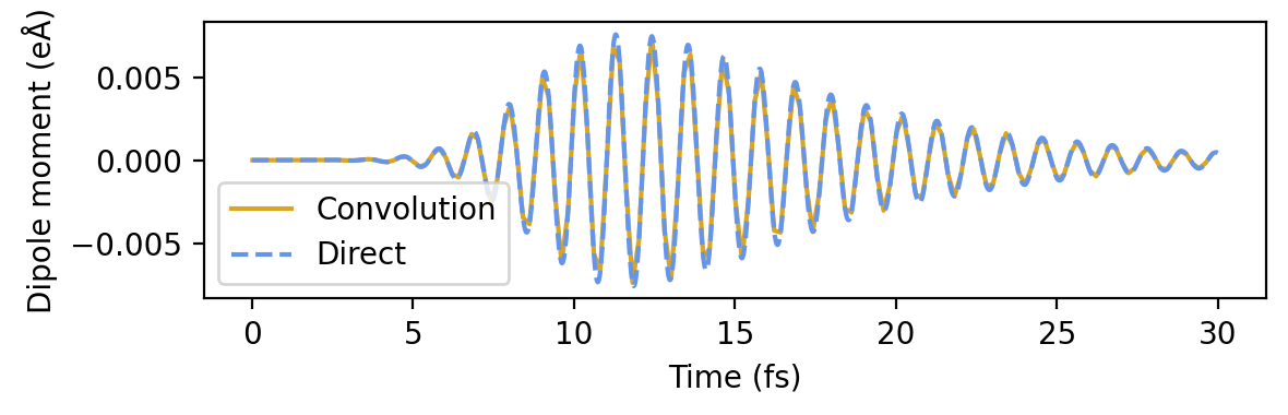
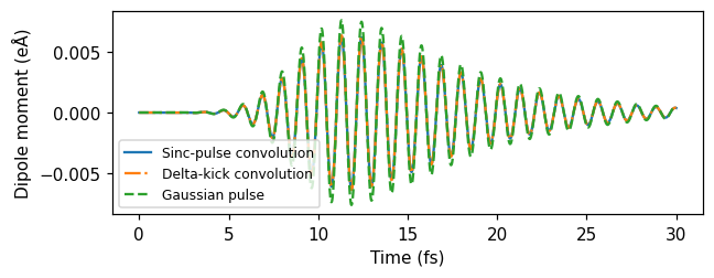
and take the inverse Fourier transform the obtain the dipole moment due to the Gaussian pulse. Plotting this quantity obtained from the sinc-pulse and delta-kick calculations, against the dipole moment from the actual Gaussian pulse calculation shows excellent agreement.

conv_from_sinc = np.fft.irfft(dipole_fourier_conv_sinc, n=padnt)[:len(times_sinc)]
conv_from_delta = np.fft.irfft(dipole_fourier_conv_delta, n=padnt)[:len(times_delta)]

# Read dipole moment from Gaussian pulse
times_gauss, dipole_moments_gauss = read_dipole_file('dm_gauss.dat')

# Plot
fig, ax = plt.subplots(1, 1, figsize=(6, 2.4))

ax.plot(times_sinc * au_to_fs, conv_from_sinc, label='Sinc-pulse convolution')
ax.plot(times_delta * au_to_fs, conv_from_delta, '-.', label='Delta-kick convolution')
ax.plot(times_gauss * au_to_fs, dipole_moments_gauss, '--', label='Gaussian pulse')

ax.set(xlabel='Time (fs)', ylabel=r'Dipole moment (eÅ)')
ax.legend(loc='lower left', fontsize=8)

fig.tight_layout()

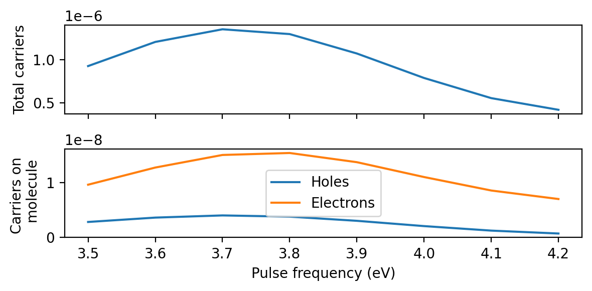
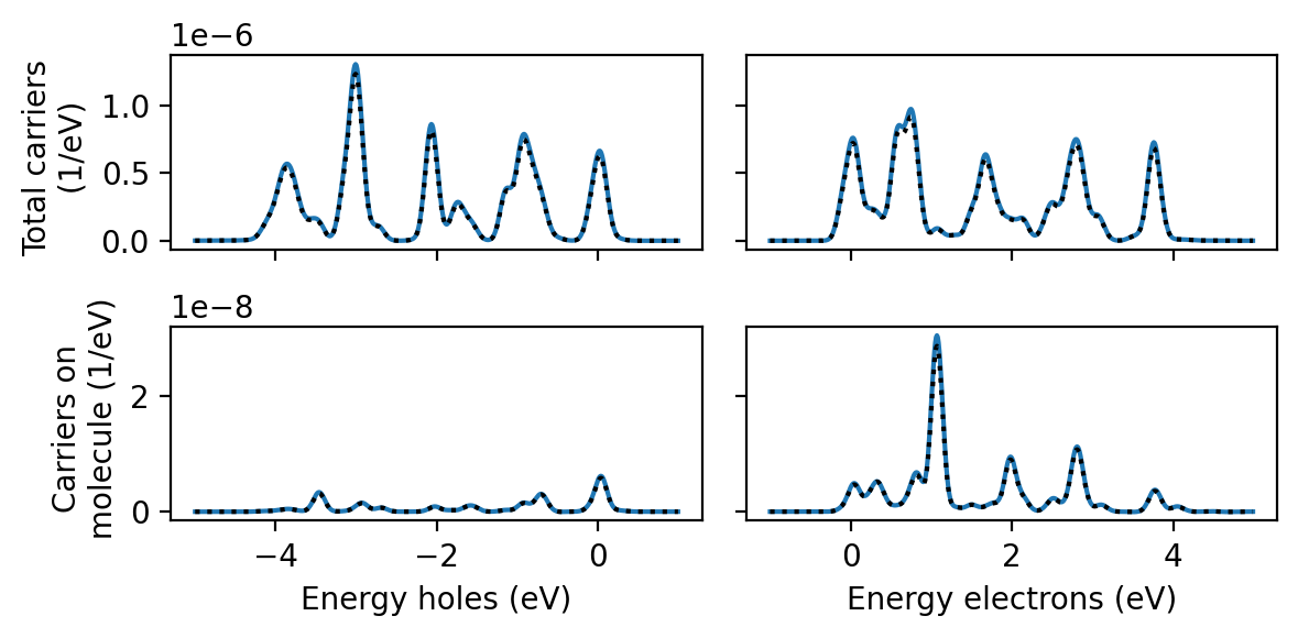
Obtaining projected hot-carrier distributions

The same principle applies to any other quantity which is linear in the perturbation, including the electron-hole part of the KS density matrix

$${\rho }_{ia}^{\text{(gauss)}}(\omega )={\rho }_{ia}^{\text{(sinc)}}(\omega )\frac{v_{\text{gauss}}(\omega )}{v_{\text{sinc}}(\omega )}.$$

We obtain projected hot-carrier distributions just like in the Getting started tutorial, with the only difference that we provide a different perturbation parameter to our ResponseFromWaveFunctions. Compared to the sinc-pulse convolution, the pulse convolution using the delta kick is drastically more expensive because the time step in the time-dependent wave functions file is 10 times shorter.

To calculate the hot-carrier distributions using the Gaussian-pulse response directly, we simply specify a perturbation=None as well as pulses=[None]. This tells rhodent to read density matrices without performing pulse convolution. This is cheap enough to run in a few minutes on a single core.

In all cases, the agreement is very good.

import numpy as np
from rhodent.response import ResponseFromWaveFunctions
from rhodent.calculators import HotCarriersCalculator
from rhodent.voronoi import VoronoiReader

# Set up the perturbation used in the TDDFT calculation
perturbation = {'name': 'deltakick', 'strength': 1e-5}

response = ResponseFromWaveFunctions(wfs_fname='wfs_delta.ulm',
                                     ksd='ksd.ulm',
                                     perturbation=perturbation)

# Set up the Gaussian pulse that we want to know the response for
pulse = {'name': 'GaussianPulse', 'strength': 1e-6,
         'frequency': 3.8, 'time0': 10e3, 'sigma': 0.3}

# Load the Voronoi weights
voronoi = VoronoiReader('voronoi.ulm')

# Set up the calculator
calc = HotCarriersCalculator(response=response,
                             voronoi=voronoi,
                             energies_occ=np.arange(-5, 1.001, 0.01),
                             energies_unocc=np.arange(-1, 5.001, 0.01),
                             sigma=0.07,
                             times=np.linspace(25e3, 30e3, 10),
                             pulses=[pulse])

# Calculate the energies
calc.calculate_distributions_and_write('hcdist_proj_delta.dat')

import numpy as np
from rhodent.response import ResponseFromWaveFunctions
from rhodent.calculators import HotCarriersCalculator
from rhodent.voronoi import VoronoiReader

# Set up a response without a perturbation specified
response = ResponseFromWaveFunctions(wfs_fname='wfs_gauss.ulm',
                                     ksd='ksd.ulm',
                                     perturbation=None)

# Load the Voronoi weights
voronoi = VoronoiReader('voronoi.ulm')

# Set up the calculator, without specifying a pulse
# No pulse convolution will be performed
calc = HotCarriersCalculator(response=response,
                             voronoi=voronoi,
                             energies_occ=np.arange(-5, 1.001, 0.01),
                             energies_unocc=np.arange(-1, 5.001, 0.01),
                             sigma=0.07,
                             times=np.linspace(25e3, 30e3, 10))

# Calculate the energies
calc.calculate_distributions_and_write('hcdist_proj_gauss.dat')

>>> Hide output <<<

>>> Show output <<<

                ###     #####
               ###############
         ########  #####     ##
     ###########            ###           _               _            _
  #######                  ###       _ __| |__   ___   __| | ___ _ __ | |_
 ####                      ##       | '__| '_ \ / _ \ / _` |/ _ \ '_ \| __|
 #                          ##      | |  | | | | (_) | (_| |  __/ | | | |_
 #                           ##     |_|  |_| |_|\___/ \__,_|\___|_| |_|\__|  0.1
 #                            ##
 #                             ##
 ##                             ###
  ####                           ###
   ##########                     ##
      ########                   ###
            ###                ####
            ##               ####
            ##           ######
            #################

Date:   Thu Mar 27 10:59:32 2025
CWD:    /home/jakub/proj/rhodent-supplementary/notebooks/pulse_convolution
cores:  1
Python: 3.12.3
numpy:  /home/jakub/git/auto-venv-setup/venv/gpaw/upstream/lib/python3.12/site-packages/numpy (version 1.26.4)
ASE:    /home/jakub/git/ase/ase (version 3.25.0b1)
GPAW:   /home/jakub/git/gpaw/upstream/gpaw (version 25.1.1b1)

[00:00:00.0] [Reader] Opening time-dependent wave functions file wfs_gauss.ulm
[00:00:00.0] [Reader] Opened time-dependent wave functions file with 150 times
[00:00:00.1] Set up calculator:
===========  HotCarriersCalculator  ============
response:
  ResponseFromWaveFunctions
    ksd: ksd.ulm
    wfs_fname: wfs_gauss.ulm
    perturbation:
      No perturbation

voronoi:
  VoronoiReader for ground state with 3626 bands
  1 projections:
    #0  : On atoms [201, 202]

Energies for broadening (sigma = 0.1 eV)
  Occupied: 601 from -5.0 to 1.0 eV
  Unoccupied: 601 from -1.0 to 5.0 eV
------------------------------------------------

==================================
 Procedure for obtaining response
==================================
Response from time-dependent wave functions

  Time-dependent wave functions reader
    Constructing density matrices in basis of ground state orbitals.

    file: wfs_gauss.ulm
      wave function dimensions (1310, 3626)
      10 times
        25020.0, 25620.0, 26220.0, ..., 29820.0 as
    1 ranks reading in 10 iterations

Density matrix shape (1123, 2521)
reading real and imaginary parts

=================
 Memory estimate
=================
Voronoi weights ii: (1, 1123, 1123) float64
. 9.6 MiB per rank on 1 ranks
. 9.6 MiB in total on all ranks

Voronoi weights aa: (1, 2521, 2521) float64
. 48.5 MiB per rank on 1 ranks
. 48.5 MiB in total on all ranks

Reading response:
    Density matrix: (1123, 2521, 2) float64
    . 43.2 MiB per rank on 1 ranks
    . 43.2 MiB in total on all ranks

    Time-dependent wave functions reader:
        C0S_nM: (1310, 3626) float64
        . 36.2 MiB per rank on 1 ranks
        . 36.2 MiB in total on all ranks

        rho0_MM: (3626, 3626) float64
        . 100.3 MiB per rank on 1 ranks
        . 100.3 MiB in total on all ranks

        ........................
        .. Total on all ranks ..
        .......136.6 MiB........

    ........................
    .. Total on all ranks ..
    .......179.7 MiB........

........................
.. Total on all ranks ..
.......237.9 MiB........

[00:00:00.3] [Reader] Constructing C0_sknM on 1 ranks
[00:00:30.0] [Reader] Constructed C0_sknM
[00:00:30.0] [Reader] Constructing rho0_skMM on 1 ranks
[00:00:47.7] [Reader] Constructed rho0_skMM
[00:00:56.2] [Calculator] Calculated and broadened HC distributions in 56.22s for 25020.0as
[00:01:04.3] [Calculator] Calculated and broadened HC distributions in 64.29s for 25620.0as
[00:01:12.3] [Calculator] Calculated and broadened HC distributions in 72.27s for 26220.0as
[00:01:20.1] [Calculator] Calculated and broadened HC distributions in 80.10s for 26820.0as
[00:01:27.9] [Calculator] Calculated and broadened HC distributions in 87.91s for 27420.0as
[00:01:35.9] [Calculator] Calculated and broadened HC distributions in 95.89s for 27820.0as
[00:01:43.7] [Calculator] Calculated and broadened HC distributions in 103.73s for 28420.0as
[00:01:51.6] [Calculator] Calculated and broadened HC distributions in 111.58s for 29020.0as
[00:02:01.0] [Calculator] Calculated and broadened HC distributions in 121.03s for 29620.0as
[00:02:08.7] [Calculator] Calculated and broadened HC distributions in 128.67s for 29820.0as
[00:02:08.7] [Calculator] Finished calculating hot-carrier matrices
[00:02:08.7] [Calculator] Written hcdist_proj_gauss.dat

>>> Hide code <<<

>>> Show code <<<

from matplotlib import pyplot as plt

data_sinc = np.loadtxt('hcdist_proj.dat')
data_delta = np.loadtxt('hcdist_proj_delta.dat')
data_gauss = np.loadtxt('hcdist_proj_gauss.dat')

fig, axes = plt.subplots(2, 1, sharex=True, figsize=(6, 4.5))

scale = 1e8
axes[0].plot(data_sinc[:, 1], scale * data_sinc[:, 3], '-')
axes[1].plot(data_sinc[:, 1], scale * data_sinc[:, 5], '-', label='Sinc-pulse convolution')

axes[0].plot(data_delta[:, 1], scale * data_delta[:, 3], '-.')
axes[1].plot(data_delta[:, 1], scale * data_delta[:, 5], '-.', label='Delta-kick convolution')

axes[0].plot(data_gauss[:, 1], scale * data_gauss[:, 3], '--')
axes[1].plot(data_gauss[:, 1], scale * data_gauss[:, 5], '--', label='Gauss response')

axes[1].legend(loc='upper left', fontsize=8)
axes[0].set_ylabel('Total carriers ($10^{-8}$/eV)')
axes[1].set_ylabel('Carriers on molecule\n($10^{-8}$/eV)')
axes[-1].set_xlabel('Energy (eV)')

fig.tight_layout()