Preparations

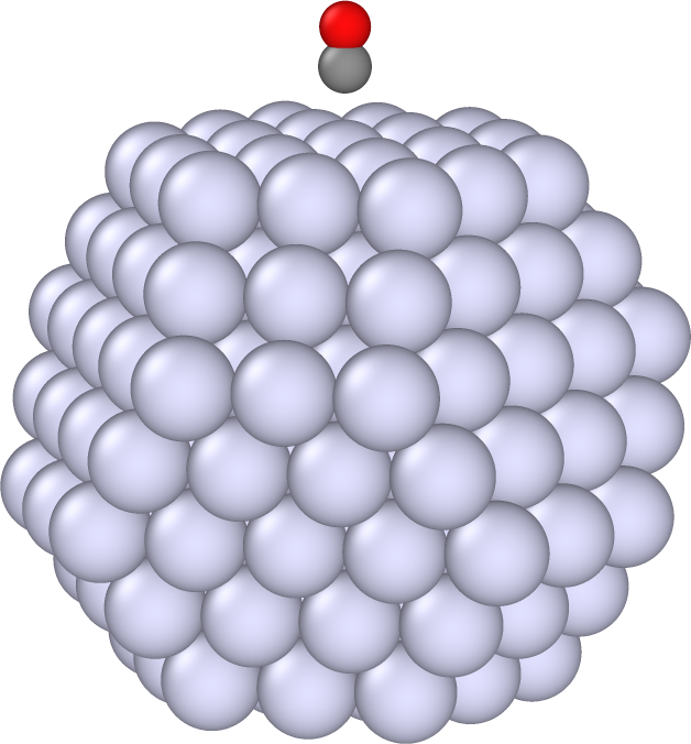
In order to use rhodent we need output from a time-dependent density functional theory (TDDFT) calculation. We set up a system consisting of a CO molecule near a plasmonic Ag nanoparticle (pictured below), and perform a real-time TDDFT calculation using GPAW.

This cells below generate files for use in other tutorials:

• Ground state calculation in GPAW

  • gs.gpw - Ground state file

• Calculation of unoccupied states in GPAW

  • gs_unocc.gpw - Ground state file including all unoccupied states

  • ksd.ulm - KohnShamDecomposition file

• Time propagation in GPAW

  • wfs.ulm - Time-dependent wave functions file

  • dm.dat - Dipole moment file

For the advanced topics, we also need:

• Time propagation with delta-kick

  • wfs_delta.ulm - Time-dependent wave functions file

  • fdm_delta.ulm - Fourier transform of density matrix file

  • dm_delta.dat - Dipole moment file

• Time propagation with Gaussian pulse

  • wfs_gauss.ulm - Time-dependent wave functions file

  • dm_gauss.dat - Dipole moment file

Note

The time propagation is very time and memory consuming. On a 32 core CPU it takes about 18 hours and requires about 100GB of memory. The resulting output files require disk space of about 11GB each for wfs.ulm and wfs_gauss.ulm, 48GB for fdm.ulm and 110GB for wfs_delta.ulm.

Ground state calculation in GPAW

The file structure.xyz contains the atomic structure of the nanoparticle-molecule system.

We read the file and set up an ground state calculation in GPAW.

• We use LCAO mode with the pvalence basis set (Kuisma et al. (2015); see here for installation).

• We use the GLLB-sc xc-functional to accurately describe the plasmonic response of Ag.

• We use a dipole-corrected Poisson solver to allow working in a smaller cell (the cell is defined in the structure file).

The configuration options and details on how to run the calculation in parallel using MPI can be found in the GPAW documentation.

from ase.io import read
from ase.parallel import parprint

from gpaw import GPAW

atoms = read('structure.xyz')

# Add dipole moment corrections to center of metallic nanoparticle
metal_i = [sym in ['Na', 'Al', 'Ag', 'Au', 'Cu'] for sym in atoms.get_chemical_symbols()]
center = atoms.get_positions()[metal_i].mean(axis=0)
parprint(f'Center of NP is at {center}', flush=True)
moment_corrections = [dict(moms=list(range(1+3)), center=center)]

calc_kwargs = {}
calc_kwargs['mode'] = 'lcao'  # LCAO mode
calc_kwargs['h'] = 0.2  # Grid spacing in Å
calc_kwargs['setups'] = {'Ag': '11'}
calc_kwargs['basis'] = {elem: 'pvalence.dz' for elem in ['Ag', 'Au', 'Cu']}
calc_kwargs['poissonsolver'] = {'name': 'MomentCorrectionPoissonSolver',
                                'moment_corrections': moment_corrections,
                                'poissonsolver': 'fast'}
calc_kwargs['mixer'] = {'beta': 0.1, 'nmaxold': 5, 'weight': 50.0}
calc_kwargs['symmetry'] = {'point_group': False}  # Necessary for RT-TDDFT
calc_kwargs['occupations'] = {'name': 'fermi-dirac', 'width': 0.05}
calc_kwargs['maxiter'] = 450
calc_kwargs['xc'] = 'GLLBSC'
calc_kwargs['txt'] = 'gs.out'
calc_kwargs['parallel'] = {'sl_auto': True,
                           'augment_grids': True,
                           'domain': 1}  # Adjust to higher value if out of memory

calc_kwargs['nbands'] = -200
calc_kwargs['convergence'] = {'density': 1e-12, 'bands': -150}

# Set up calculator and converge ground state
calc = GPAW(**calc_kwargs)

atoms.calc = calc
atoms.get_potential_energy()

# Write the ground state to file
calc.write('gs.gpw', mode='all')

Calculation of unoccupied states in GPAW

For later analysis, we will need to compute the Kohn-Sham (KS) wave functions in the full space, including all unoccupied states. We also construct a KohnShamDecomposition object to hold some additional information, like the dipole operator in the KS basis.

from ase.parallel import parprint
from gpaw import GPAW
from gpaw.lcaotddft.ksdecomposition import KohnShamDecomposition

gpwfile = 'gs.gpw'
gsunoccfile = 'gs_unocc.gpw'
ksdfile = 'ksd.ulm'

# Calculate ground state with full unoccupied space
parprint('Loading GS with full unoccupied space', flush=True)
calc = GPAW(gpwfile, fixdensity=True, nbands='nao')

calc.get_potential_energy()

parprint(f'Saving GS with full unoccupied space to {gsunoccfile}', flush=True)
calc.write(gsunoccfile, mode='all')

# Construct KS electron-hole basis
ksd = KohnShamDecomposition(calc)
ksd.initialize(calc)
ksd.write(ksdfile)
parprint(f'Saving Kohn-Sham decomposition to {ksdfile}', flush=True)

Time propagation in GPAW

Now we load the ground state file (the first file, with only the occupied states), perturb the system, and perform time propagation for 30 fs. We use a weak, temporally sinc-shaped laser pulse with a spatially uniform spatial profile as the perturbation. This is essentially similar to a delta-kick, with the added advantage that only low-frequency components of the response are probed. A smooth cut-off at 8 eV is chosen. For more information about the sinc-pulse see the in depth tutorial The convolution trick.

The time propagation is our most time consuming task. It is highly advisable to split the calculation into several shorter running jobs by writing to a restart file, and later restarting. We refer to the GPAW documentation on how to run using MPI and restart files.

• We attach a DipoleMomentWriter that writes the dipole moment at every timestep to dm.dat

• We attach a WaveFunctionWriter that writes the time-dependent wave functions to wfs.ulm. To save disk space, we write it every 10 steps (0.2 fs, corresponding to a Nyquist frequency of about 10 eV).

• We start 1500 propagation steps of 20 as, for a total of 30 fs propagation time.

from ase.units import Hartree, Bohr
from gpaw.external import ConstantElectricField
from gpaw.lcaotddft import LCAOTDDFT
from gpaw.lcaotddft.dipolemomentwriter import DipoleMomentWriter
from gpaw.lcaotddft.laser import create_laser
from gpaw.lcaotddft.wfwriter import WaveFunctionWriter


# Temporal shape of the time-dependent potential
pulse = {'name': 'SincPulse',
         'strength': 1e-6,  # Amplitude
         'cutoff_freq': 8,  # Cut-off frequency in units of eV
         'time0': 5,  # Time of maximum in number of oscillations
         'relative_t0': True}
# Spatial shape of the time-dependent potential
ext = ConstantElectricField(Hartree / Bohr, [0., 0., 1.])
# Time-dependent potential
td_potential = {'ext': ext, 'laser': create_laser(pulse)}

# Set up the time-propagation calculation
td_calc = LCAOTDDFT('gs.gpw',
                    td_potential=td_potential,
                    parallel={'sl_auto': True,
                              'augment_grids': True,
                              'domain': 1},  # Adjust to higher value if out of memory
                    txt='td.out')

# Attach the data recording and analysis tools
DipoleMomentWriter(td_calc, 'dm.dat')
WaveFunctionWriter(td_calc, 'wfs.ulm', interval=10)

# Propagate
td_calc.propagate(20, 1500)

Time propagation with delta-kick

A more conventional perturbation in real-time TDDFT is the delta-kick. In The convolution trick we show that we can obtain the same results using the delta-kick, sinc-shaped pulse and Gaussian pulse.

Because the delta-kick induces all frequency responses, we can no longer write the time-dependent wave functions file using a sparse interval, as this would introduce aliasing from the high frequencies.

• We attach a WaveFunctionWriter that writes the time-dependent wave functions to wfs_delta.ulm at every time step.

• We set up a FrequencyDensityMatrix that is set to compute the Fourier transform of the density matrices iteratively during propagation. After finishing the propagation, we write it to disk fdm.ulm. A grid of frequencies up to 6 eV is saved, with a frequency spacing of 50meV.

As previously, we also attach the DipoleMomentWriter that writes the dipole moment at every timestep to dm_delta.dat.

Note

rhodent only needs one of the WaveFunctionWriter or FrequencyDensityMatrix to calculate the response. Here we save both for the purpose of comparison.

Warning

The frequency spacing of 50meV in the grid for the Fourier transform corresponds to a Nyquist time of about 41 fs. If we propagate for longer than 41 fs we will see effects of aliasing, and our data will be ruined. Care must be taken to increase the frequency grid if we want longer propagation times.

import numpy as np
from gpaw.lcaotddft import LCAOTDDFT
from gpaw.lcaotddft.densitymatrix import DensityMatrix
from gpaw.lcaotddft.dipolemomentwriter import DipoleMomentWriter
from gpaw.lcaotddft.frequencydensitymatrix import FrequencyDensityMatrix
from gpaw.tddft.folding import frequencies
from gpaw.lcaotddft.wfwriter import WaveFunctionWriter


# Set up the time-propagation calculation
td_calc = LCAOTDDFT('gs.gpw',
                    parallel={'sl_auto': True,
                              'augment_grids': True,
                              'domain': 1},  # Adjust to higher value if out of memory
                    txt='td_delta.out')

# Attach the data recording and analysis tools
dmat = DensityMatrix(td_calc)
freqs = frequencies(np.arange(0.05, 6.01, 0.05), None, None)
fdm = FrequencyDensityMatrix(td_calc, dmat, frequencies=freqs)

# Attach the data recording and analysis tools
DipoleMomentWriter(td_calc, 'dm_delta.dat')
WaveFunctionWriter(td_calc, 'wfs_delta.ulm')

# Kick
td_calc.absorption_kick([0, 0, 1e-5])

# Propagate
td_calc.propagate(20, 1500)

# Write Fourier transform of density matrix
fdm.write('fdm_delta.ulm')

Time propagation with Gaussian pulse

If we are interested in the response to a Gaussian pulse, we can simply apply this pulse directly in the real-time TDDFT calculation. In The convolution trick we show that we can obtain the same results using the delta-kick, sinc-shaped pulse and Gaussian pulse.

We set up a Gausian pulse with frequency 3.8 eV, time of maximum amplitude 10 fs.

• We attach a DipoleMomentWriter that writes the dipole moment at every timestep to dm_gauss.dat

• We attach a WaveFunctionWriter that writes the time-dependent wave functions to wfs_gauss.ulm. To save disk space, we write it every 10 steps (0.2 fs).

from ase.units import Hartree, Bohr
from gpaw.external import ConstantElectricField
from gpaw.lcaotddft import LCAOTDDFT
from gpaw.lcaotddft.dipolemomentwriter import DipoleMomentWriter
from gpaw.lcaotddft.laser import create_laser
from gpaw.lcaotddft.wfwriter import WaveFunctionWriter


# Temporal shape of the time-dependent potential
pulse = {'name': 'GaussianPulse',
         'strength': 1e-6,
         'frequency': 3.8,
         'time0': 10e3,
         'sigma': 0.3,
         'sincos': 'cos'}
# Spatial shape of the time-dependent potential
ext = ConstantElectricField(Hartree / Bohr, [0., 0., 1.])
# Time-dependent potential
td_potential = {'ext': ext, 'laser': create_laser(pulse)}

# Set up the time-propagation calculation
td_calc = LCAOTDDFT('gs.gpw',
                    td_potential=td_potential,
                    parallel={'sl_auto': True,
                              'augment_grids': True,
                              'domain': 1},  # Adjust to higher value if out of memory
                    txt='td_gauss.out')

# Attach the data recording and analysis tools
DipoleMomentWriter(td_calc, 'dm_gauss.dat')
WaveFunctionWriter(td_calc, 'wfs_gauss.ulm', interval=10)

# Propagate
td_calc.propagate(20, 1500)

References

• 13. Kuisma, A. Sakko, T. P. Rossi, A. H. Larsen, J. Enkovaara, L. Lehtovaara, and T. T. Rantala, Localized surface plasmon resonance in silver nanoparticles: Atomistic first-principles time-dependent density-functional theory calculations, Phys. Rev. B 91, 115431 (2015).