Getting started
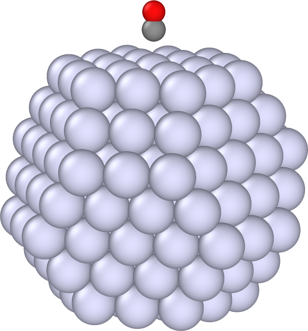
In this tutorial we use rhodent to obtain hot-carrier distributions and other observables. We study a CO molecule near a plasmonic Ag nanoparticle (pictured below). As a starting point, we need output from a real-time time-dependent density functional theory (TDDFT) calculation, which we perform using GPAW. Follow the steps in Preparations to obtain the following files:
gs_unocc.gpw- Ground state file including all unoccupied statesksd.ulm- KohnShamDecomposition filewfs.ulm- Time-dependent wave functions filedm.dat- Dipole moment file
Calculating the spectrum
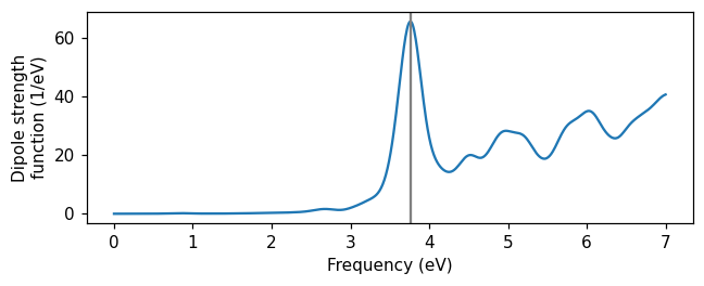
The first thing we want to know about our system is what frequency the plasmonic resonance has. We use the SpectrumCalculator, giving it the name of the dipole moment file and the type of perturbation used in the TDDFT calculation. We calculate the spectrum on a frequency grid between 0 and 7 eV using Gaussian broadening with a width parameter of 0.1 eV, and save the spectrum to a text file spectrum.dat. Some
additional information about the simulation and broadening is printed in the header of the file, which we see upon inspection.
Plotting the spectrum, we see a clear peak at about 3.8 eV. This corresponds to the localized surface plasmon resonance of the small Ag nanoparticle.
[ ]:
import numpy as np
from rhodent.spectrum import SpectrumCalculator

# Set up the perturbation used in the TDDFT calculation
perturbation = {'name': 'SincPulse', 'strength': 1e-6, 'cutoff_freq': 8,
                'time0': 5, 'relative_t0': True}

# Set up the spectrum calculator
calc = SpectrumCalculator.from_file('dm.dat',
                                    perturbation=perturbation)

# Calculate the spectrum
calc.calculate_spectrum_and_write('spectrum.dat',
                                  frequencies=np.arange(0, 7.001, 0.01),
                                  frequency_broadening=0.1)
Written spectrum.dat
[ ]:
!head 'spectrum.dat'
# Photoabsorption spectrum from real-time propagation
# Calculated using rhodent version: 0.1
# Total time = 30.0000 fs, Time steps = 20.00 as
# Perturbation during calculation was:
#   name: SincPulse, strength: 1e-06, time0: 5
#   cutoff_freq: 8, relative_t0: True
# Gaussian broadening width 0.10 eV
#    om (eV)           S_x (1/eV)           S_y (1/eV)           S_z (1/eV)
    0.000000     0.0000000000e+00     0.0000000000e+00     0.0000000000e+00
    0.010000     7.4613605737e-08     2.9198928622e-09    -2.2737690069e-06
[ ]:
import numpy as np
from matplotlib import pyplot as plt

fig, ax = plt.subplots(1, 1, figsize=(6, 2.5))

# Plot z-component
frequency, _, _, osc = np.loadtxt('spectrum.dat', unpack=True)

ax.plot(frequency, osc)
ax.axvline(3.76, color='grey')
ax.set_xlabel('Frequency (eV)')
ax.set_ylabel('Dipole strength\nfunction (1/eV)')

fig.tight_layout()
Calculating a transition contribution map
The spectrum can be written as a sum of matrix elements
in the basis of ground state Kohn-Sham orbitals. The elements are related to the elements of the Kohn-Sham density matrix. For more details, see the documentation of DipoleCalculator. Each element corresponds to a transition that leaves a hole in occupied state
In a transition contribution map (TCM), the elements are broadened on two energy grids (for occupied and unoccupied orbitals respectively)
by convolution with Gaussians
Using rhodent, we can calculate the spectrum TCM by setting up a DipoleCalculator. The calculator needs:
A Response object, which describes how the Kohn-Sham density matrix can be obtained. In our case it is using the time-dependent wave functions file
wfs.ulm, which means that we use the ResponseFromWaveFunctions. The response also needs the KohnShamDecomposition fileksd.ulmand the perturbation.Frequency grids for occupied and unoccupied energies. We choose -5 eV to 1 eV, and -1 eV to 5 eV.
A Gaussian broadening parameter
Frequencies at which to compute the spectrum, we choose the peak at 3.8 eV.
In order to be consistent with the spectrum calculation from the dipole moment file, we also apply a Gaussian broadening parameter of 0.1 eV for the frequencies.
To compute the TCM, we call the calculate_and_write function. The include_tcm argument is needed to actually compute the TCM (otherwise just the polarizability is computed). We save the data in a zipped numpy archive by providing a file name with the .npz extension.
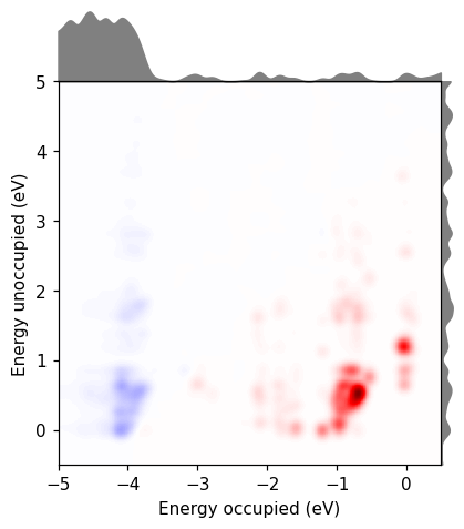
We can also use rhodent to calculate the density of states (DOS) from the gs_unocc.gpw file using DOSCalculator. Plotting the DOS together with the TCM reveals that most of the contribution to the spectrum comes from transitions near the Fermi level, just like the textbook picture of a plasmon. There are also destructive contributions from occupied states around -4 eV. This is the screening from the d-type orbitals.
[ ]:
import numpy as np
from rhodent.response import ResponseFromWaveFunctions
from rhodent.calculators import DipoleCalculator

# Set up the perturbation used in the TDDFT calculation
perturbation = {'name': 'SincPulse', 'strength': 1e-6, 'cutoff_freq': 8,
                'time0': 5, 'relative_t0': True}

response = ResponseFromWaveFunctions(wfs_fname='wfs.ulm',
                                     ksd='ksd.ulm',
                                     perturbation=perturbation)

calc = DipoleCalculator(response=response,
                        energies_occ=np.arange(-5, 1.001, 0.01),
                        energies_unocc=np.arange(-1, 5.001, 0.01),
                        sigma=0.07,
                        frequencies=[3.8],
                        frequency_broadening=0.1)

# Calculate the dipole contributions
calc.calculate_and_write('tcm.npz', include_tcm=True)
[ ]:
!unzip -l tcm.npz # List the archive contents
Archive:  tcm.npz
  Length      Date    Time    Name
---------  ---------- -----   ----
    29136  1980-01-01 00:00   eig_n.npy
     9112  1980-01-01 00:00   eig_i.npy
    20296  1980-01-01 00:00   eig_a.npy
      136  1980-01-01 00:00   imin.npy
      136  1980-01-01 00:00   imax.npy
      136  1980-01-01 00:00   amin.npy
      136  1980-01-01 00:00   amax.npy
      136  1980-01-01 00:00   sigma.npy
     4936  1980-01-01 00:00   energy_o.npy
     4936  1980-01-01 00:00   energy_u.npy
      136  1980-01-01 00:00   freq_w.npy
      136  1980-01-01 00:00   frequency_broadening.npy
      136  1980-01-01 00:00   osc_prefactor_w.npy
      176  1980-01-01 00:00   dm_wv.npy
 17337776  1980-01-01 00:00   dm_wouv.npy
      128  1980-01-01 00:00   dm_proj_wIIv.npy
      128  1980-01-01 00:00   atom_projections.npy
---------                     -------
 17407712                     17 files
[ ]:
from rhodent.dos import DOSCalculator

calc = DOSCalculator.from_gpw(gpw_file='gs_unocc.gpw',
                              voronoi=None,
                              energies=np.arange(-5, 5.001, 0.01),
                              sigma=0.07,
                              zerofermi=True)
calc.calculate_dos_and_write('dos.dat')
[00:00:00.1] [Calculator] Computed DOS
[00:00:00.1] [Calculator] Written dos.dat
[ ]:
!head dos.dat
# DOS relative to Fermi level
# Gaussian folding, Width 0.0700 eV
# Energy (eV)        DOS (1/eV)
   -5.000000     3.07811837e+02
   -4.990000     3.10586059e+02
   -4.980000     3.13661189e+02
   -4.970000     3.17037193e+02
   -4.960000     3.20718871e+02
   -4.950000     3.24711448e+02
   -4.940000     3.29013729e+02
[ ]:
import numpy as np
from matplotlib import pyplot as plt
from matplotlib.colors import Normalize

# Load the density of states
energy_e, dos_e = np.loadtxt('dos.dat', unpack=True)

# Load the transition contribution map
archive = np.load('tcm.npz')

osc_ou = archive['dm_wouv'][0, :, :, 2].imag * archive['osc_prefactor_w'][0]
energy_o = archive['energy_o']
energy_u = archive['energy_u']

# Setup axis
fig, ax = plt.subplots(1, 1, figsize=(6, 4.5))

vmax = np.max(np.abs(osc_ou))
norm = Normalize(-vmax, vmax)

# Plot the transition contribution map
ax.pcolormesh(energy_o, energy_u, osc_ou.T, cmap='seismic', norm=norm)

# Plot a normalized density of states outside the axes
dos_e /= dos_e.max()
ax.fill_between(energy_e[energy_e < 0.5], 5 + dos_e[energy_e < 0.5], 5, color='grey', clip_on=False)
ax.fill_betweenx(energy_e[energy_e > -0.5], 0.5 + dos_e[energy_e > -0.5], 0.5, color='grey', clip_on=False)

ax.set_aspect('equal',adjustable='box')
ax.set_xlim([-5, 0.5])
ax.set_ylim([-0.5, 5])

ax.set_xlabel('Energy occupied (eV)')
ax.set_ylabel('Energy unoccupied (eV)')

fig.tight_layout()
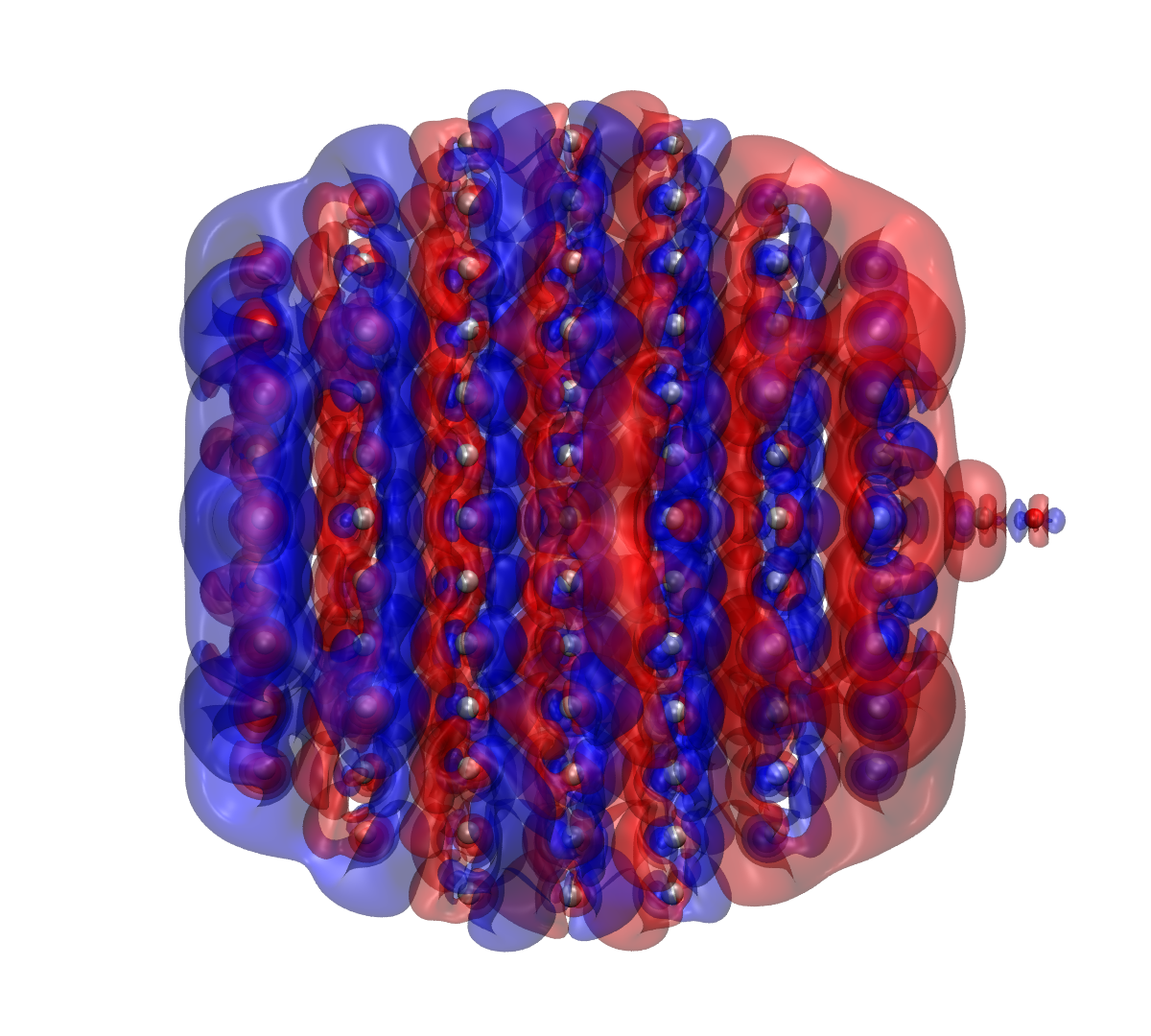
Calculating the induced density
We can also visualize the induced density contributing to the spectrum using the DensityCalculator.
Besides the response, the list of frequencies, and a value for the Gaussian broadening parameter, this calculator additionally needs the file name of the ground state file.
We use the calculate_and_write function to save a cube file, which can be plotted using a software for 3D visualization. The rendered image nicely shows the dipolar density due to the plasmon in the nanoparticle. We can also see regions of opposite charge around each atom due to the d-electron screening.
[ ]:
from rhodent.response import ResponseFromWaveFunctions
from rhodent.calculators import DensityCalculator

# Set up the perturbation used in the TDDFT calculation
perturbation = {'name': 'SincPulse', 'strength': 1e-6, 'cutoff_freq': 8,
                'time0': 5, 'relative_t0': True}

response = ResponseFromWaveFunctions(wfs_fname='wfs.ulm',
                                     ksd='ksd.ulm',
                                     perturbation=perturbation)

calc = DensityCalculator(gpw_file='gs_unocc.gpw',
                         response=response,
                         frequencies=[3.8],
                         frequency_broadening=0.1)

# Calculate the induced density
calc.calculate_and_write('plasmon.cube', which='induced')
Calculating the response to Gaussian laser
Now that we know that our system has a resonance at 3.8 eV, we wonder how its time evolution looks if we drive it with a laser pulse centered at 3.8 eV.
Using rhodent, we can take advantage of the pulse convolution trick, where we take the response from one perturbation (the sinc-pulse) and transform it into the response to another perturbation (a Gaussian pulse). The details of the pulse convolution are described in The convolution trick.
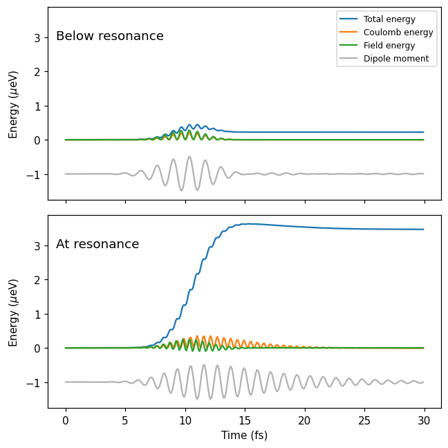
We set up the perturbation and response object like before, and use the EnergyCalculator to compute the time-evolution of energies after the new perturbation. The calculator needs, besides the response object:
An array of times. We choose a dense array from the beginning to the end of the simulation.
One or several pulses. Computing the response to several pulses takes only marginally more time than to one pulse, so we might as well set up a pulse resonant with the plasmon (3.8 eV) and one off-resonant (3.0 eV). The pulses are about 5 fs in duration and peak at 10 fs simulation time.
Plotting the energies, we see that, after resonant excitation, a plasmon forms in the system. The plasmon persists for about 10 fs after the decay of the pulse, revealed by the oscillating dipole moment and Coulomb energy. Excitation below the resonance, however, does not leave any oscillations in the system after the pulse decay.
[ ]:
import numpy as np
from rhodent.response import ResponseFromWaveFunctions
from rhodent.calculators import EnergyCalculator

# Set up the perturbation used in the TDDFT calculation
perturbation = {'name': 'SincPulse', 'strength': 1e-6, 'cutoff_freq': 8,
                'time0': 5, 'relative_t0': True}

response = ResponseFromWaveFunctions(wfs_fname='wfs.ulm',
                                     ksd='ksd.ulm',
                                     perturbation=perturbation)

# Set up the Gaussian pulse that we want to know the response for
pulses = [{'name': 'GaussianPulse', 'strength': 1e-6,
           'frequency': freq, 'time0': 10e3, 'sigma': 0.3}
          for freq in [3.0, 3.8]]

# Set up the calculator
calc = EnergyCalculator(response=response,
                        times=np.linspace(0, 30e3, 301),
                        pulses=pulses)

# Calculate the energies
calc.calculate_and_write('energy.npz', only_one_pulse=False)
[ ]:
!unzip -l energy.npz # List the archive contents
Archive:  energy.npz
  Length      Date    Time    Name
---------  ---------- -----   ----
    29136  1980-01-01 00:00   eig_n.npy
     9112  1980-01-01 00:00   eig_i.npy
    20296  1980-01-01 00:00   eig_a.npy
      136  1980-01-01 00:00   imin.npy
      136  1980-01-01 00:00   imax.npy
      136  1980-01-01 00:00   amin.npy
      136  1980-01-01 00:00   amax.npy
     2528  1980-01-01 00:00   time_t.npy
      144  1980-01-01 00:00   pulsefreq_p.npy
      144  1980-01-01 00:00   pulsefwhm_p.npy
     4928  1980-01-01 00:00   dm_pt.npy
     4928  1980-01-01 00:00   total_pt.npy
     4928  1980-01-01 00:00   total_Hxc_pt.npy
     4928  1980-01-01 00:00   Epulse_pt.npy
      128  1980-01-01 00:00   total_proj_ptII.npy
      128  1980-01-01 00:00   total_Hxc_proj_ptII.npy
      128  1980-01-01 00:00   atom_projections.npy
---------                     -------
    82000                     17 files
[ ]:
import numpy as np
from matplotlib import pyplot as plt

archive = np.load('energy.npz')

fig, axes = plt.subplots(2, 1, figsize=(6, 6), sharex=True, sharey=True)
for p, ax in enumerate(axes):
    ax.plot(archive['time_t'], 1e6 * archive['total_pt'][p], label='Total energy')
    ax.plot(archive['time_t'], 1e6 * archive['total_Hxc_pt'][p], label='Coulomb energy')
    ax.plot(archive['time_t'], 1e6 * archive['Epulse_pt'][p], label='Field energy')
    dm_t = archive['dm_pt'][p]
    ax.plot(archive['time_t'], -1 + 0.5 * dm_t / dm_t.max(), color='0.7', label='Dipole moment')
ax.set_xlabel('Time (fs)')
axes[0].set_ylabel(r'Energy ($\mu$eV)')
axes[1].set_ylabel(r'Energy ($\mu$eV)')
axes[0].set_title('Below resonance', x=0.02, y=0.85, va='top', ha='left')
axes[1].set_title('At resonance', x=0.02, y=0.85, va='top', ha='left')
axes[0].legend(fontsize=8)

fig.tight_layout()
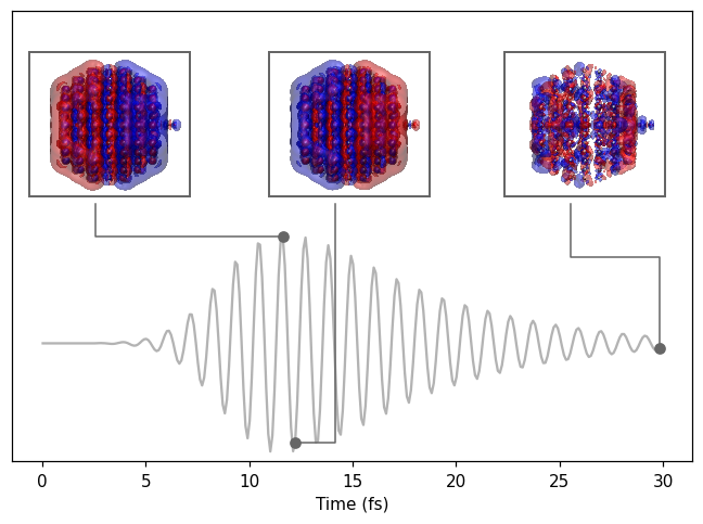
Calculating the density
The DensityCalculator also works in the time domain. We can use it like before, exchanging the frequencies and frequency_broadening arguments for times and pulses.
Rendering the density at a few selected times reaveals the dipolar density during the lifetime of the plasmon. At the end of the simulation, the plasmon has dephased.
[ ]:
import numpy as np
from rhodent.response import ResponseFromWaveFunctions
from rhodent.calculators import DensityCalculator

# Set up the perturbation used in the TDDFT calculation
perturbation = {'name': 'SincPulse', 'strength': 1e-6, 'cutoff_freq': 8,
                'time0': 5, 'relative_t0': True}

response = ResponseFromWaveFunctions(wfs_fname='wfs.ulm',
                                     ksd='ksd.ulm',
                                     perturbation=perturbation)

pulse = {'name': 'GaussianPulse', 'strength': 1e-6,
         'frequency': 3.8, 'time0': 10e3, 'sigma': 0.3}

calc = DensityCalculator(gpw_file='gs_unocc.gpw',
                         response=response,
                         pulses=[pulse],
                         times=[11.6e3, 12.1e3, 30e3])

# Calculate the induced density
calc.calculate_and_write('density_t{time:09.1f}.cube', which='induced')
Analyzing the hot-carrier distributions
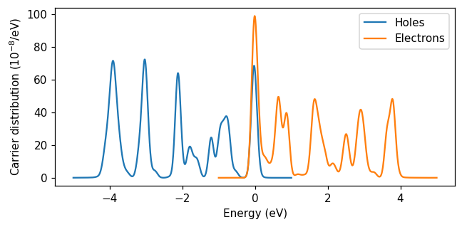
After 30 fs of simulation time, the energy is no longer in the plasmon. Instead, there is a non-thermal distribution of excited electrons and holes (often referred to as hot carriers). We calculate the hot-carrier distribution using the HotCarriersCalculator.
We initialize the calculator with a resonant pulse, and give it a list of times between 25 fs and 30 fs. Just like for the TCM calculation, we give the calculator two energy grids – one for occupied states (holes) and one for unoccupied states (electrons). Using the calculate_distributions_and_write function, the carrier distributions are computed and saved to a text file. By default, this function averages the distributions for the times given to the calculator.
We see that hot carriers at various energies up to the pulse frequency are created in the nanoparticle. Every hole in an occupied state corresponds to an electron in an unoccupied state, and their energy difference should be equal to the pulse frequency. Therefore, the distribution of electrons looks like a shifted image of the distribution of holes. Of course, the Gaussian pulse we used has a finite width (of about 0.7 eV at half maximum) so the electron and hole distributions are not exact images of each other.
Because the ground state has finite occupation number smearing, there are partially occupied states, which is why we have both electrons and holes at 0 eV.
We should also keep in mind that by using an electric field of
[ ]:
import numpy as np
from rhodent.response import ResponseFromWaveFunctions
from rhodent.calculators import HotCarriersCalculator

# Set up the perturbation used in the TDDFT calculation
perturbation = {'name': 'SincPulse', 'strength': 1e-6, 'cutoff_freq': 8,
                'time0': 5, 'relative_t0': True}

response = ResponseFromWaveFunctions(wfs_fname='wfs.ulm',
                                     ksd='ksd.ulm',
                                     perturbation=perturbation)

# Set up the Gaussian pulse that we want to know the response for
pulse = {'name': 'GaussianPulse', 'strength': 1e-6,
         'frequency': 3.8, 'time0': 10e3, 'sigma': 0.3}

# Set up the calculator
calc = HotCarriersCalculator(response=response,
                             energies_occ=np.arange(-5, 1.001, 0.01),
                             energies_unocc=np.arange(-1, 5.001, 0.01),
                             sigma=0.07,
                             times=np.linspace(25e3, 30e3, 10),
                             pulses=[pulse])

# Calculate the energies
calc.calculate_distributions_and_write('hcdist.dat')
[ ]:
!head hcdist.dat
# Hot carrier (H=hole, E=electron) distributions relative to Fermi level
# Response to pulse with frequency 3.80eV, FWHM 5.17fs
# Averaged for 10 times between 25.0fs-29.8fs
# Gaussian folding, Width 0.0700eV
# H energy (eV)   E energy (eV)     Total H (1/eV)     Total E (1/eV)
      -5.000000       -1.000000     3.17848274e-10     1.51359390e-46
      -4.990000       -0.990000     3.24229460e-10     1.01897872e-45
      -4.980000       -0.980000     3.30580262e-10     6.72168734e-45
      -4.970000       -0.970000     3.36919572e-10     4.34460106e-44
      -4.960000       -0.960000     3.43287380e-10     2.75157212e-43
[ ]:
from matplotlib import pyplot as plt

fig, ax = plt.subplots(1, 1, figsize=(6, 3))

data = np.loadtxt('hcdist.dat')
energies_occ = data[:, 0]
energies_unocc = data[:, 1]

scale = 1e8
hcdist_o = data[:, 2]
hcdist_u = data[:, 3]
ax.plot(energies_occ, scale * hcdist_o, label='Holes')
ax.plot(energies_unocc, scale * hcdist_u, label='Electrons')

ax.set_ylabel('Carrier distribution ($10^{-8}$/eV)')
ax.set_xlabel('Energy (eV)')
ax.legend()

fig.tight_layout()
Where are the hot carriers localized?
We can also compute projected hot-carrier distributions using rhodent. We compute a matrix of Voronoi weights corresponding to pairs of ground state orbitals
where the intergral is taken in the Voronoi partition of one or several atoms in space. For the diagonals
We compute the Voronoi weights for the CO molecule (atoms numbered 201 and 202) using the VoronoiWeightCalculator. We could pass the Voronoi calculator directly to the HotCarriers calculator the compute the weights on the fly, but as this is very memory intensive, it is recommended to first save them to a file voronoi.ulm using
calculate_and_write Then we load the voronoi weights using the VoronoiReader and pass it to the HotCarriersCalculator.
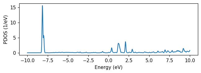
To visualize the weights, we compute a partial DOS using the DOSCalculator with the VoronoiReader. Plotting it, we see the highest occupied molecular orbital about 8 eV below the Fermi level. Being further from the Fermi level than the pulse frequency, we should expect few holes to form in the molecule. The lowest unoccupied molecular orbital (LUMO) is strongly hybridized with the metal surface, with several peaks between 0 and 3 eV above the Fermi level. It should thus be possible for electrons to be excited from the nanoparticle to the moleucle by the laser pulse.
[ ]:
from rhodent.voronoi import VoronoiWeightCalculator

voronoi = VoronoiWeightCalculator.from_gpw([[201, 202]], 'gs_unocc.gpw')
voronoi.calculate_and_write('voronoi.ulm')
[ ]:
from rhodent.dos import DOSCalculator
from rhodent.voronoi import VoronoiReader

# Load the Voronoi weights
voronoi = VoronoiReader('voronoi.ulm')

calc = DOSCalculator.from_gpw(gpw_file='gs_unocc.gpw',
                              voronoi=voronoi,
                              energies=np.arange(-10, 10.001, 0.01),
                              sigma=0.05,
                              zerofermi=True)
calc.calculate_pdos_and_write('pdos.dat')
[00:00:00.1] [Calculator] Computed gaussians
[00:00:00.1] [Calculator] Computed PDOS for projection [201, 202]
[00:00:00.1] [Calculator] Written pdos.dat
[ ]:
!head pdos.dat
# PDOS relative to Fermi level
# Atomic projections:
#      0: [201, 202]
# Gaussian folding, Width 0.0500 eV
# Energy (eV)   PDOS    0 (1/eV)
   -10.000000     3.18922897e-57
    -9.990000     1.21076200e-58
    -9.980000     4.41631545e-60
    -9.970000     1.54771008e-61
    -9.960000     5.21131538e-63
[ ]:
from matplotlib import pyplot as plt

energies, pdos = np.loadtxt('pdos.dat', unpack=True)

fig, ax = plt.subplots(1, 1, figsize=(6, 2.25))

ax.plot(energies, pdos)
ax.set(xlabel='Energy (eV)', ylabel='PDOS (1/eV)')

fig.tight_layout()
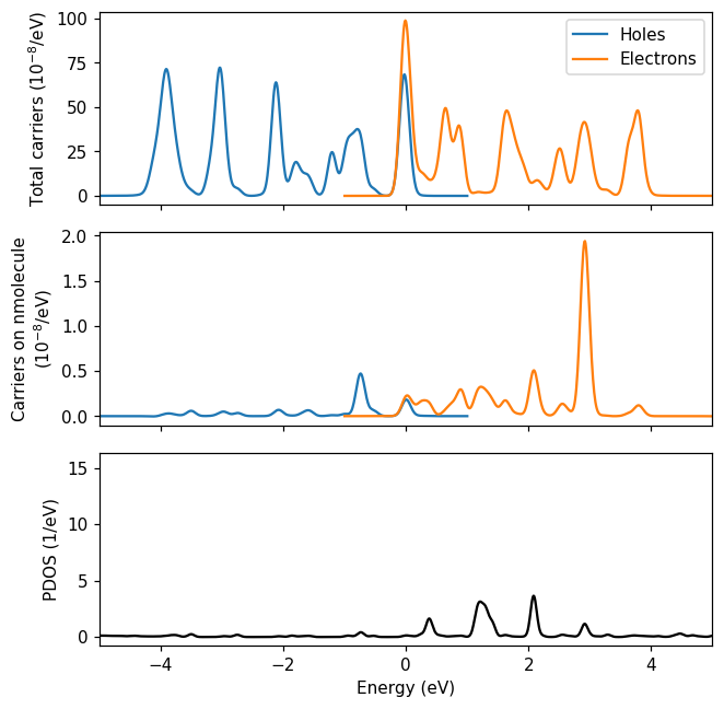
Passing the VoronoiReader to the HotCarriersCalculator we compute projected hot-carrier distributions (refer to the documentation of the latter for a description of the projection). An additional set of columns corresponding to projected hot-carrier distributions are written to the text file. Plotting the data, we confirm that there is almost no hole transfer to the molecule. The number of electrons in the molecule amounts to a few percent of the amount of electrons in the system as a whole, which is natural since the nanoparticle is much bigger than the molecule. Interestingly, the amount of electrons in each of the hybridized LUMO states is not simply proportional to the PDOS weight. The amount of electron transfer is determined by a combination of energies of possible donor states in the nanoparticle, the hybridized LUMO and the pulse frequency (Fojt et al. (2022)).
Note
It is also possible to omit the step of writing the Voronoi weights to disk and later reading them. Simply pass the VoronoiWeightCalculator as an argument to the HotCarriersCalculator and the Voronoi weights are computed on the fly. This, however, is very memory intensive when running in parallel.
[ ]:
import numpy as np
from rhodent.response import ResponseFromWaveFunctions
from rhodent.calculators import HotCarriersCalculator
from rhodent.voronoi import VoronoiReader

# Set up the perturbation used in the TDDFT calculation
perturbation = {'name': 'SincPulse', 'strength': 1e-6, 'cutoff_freq': 8,
                'time0': 5, 'relative_t0': True}

response = ResponseFromWaveFunctions(wfs_fname='wfs.ulm',
                                     ksd='ksd.ulm',
                                     perturbation=perturbation)

# Set up the Gaussian pulse that we want to know the response for
pulse = {'name': 'GaussianPulse', 'strength': 1e-6,
         'frequency': 3.8, 'time0': 10e3, 'sigma': 0.3}

# Load the Voronoi weights
voronoi = VoronoiReader('voronoi.ulm')

# Set up the calculator
calc = HotCarriersCalculator(response=response,
                             voronoi=voronoi,
                             energies_occ=np.arange(-5, 1.001, 0.01),
                             energies_unocc=np.arange(-1, 5.001, 0.01),
                             sigma=0.07,
                             times=np.linspace(25e3, 30e3, 10),
                             pulses=[pulse])

# Calculate the energies
calc.calculate_distributions_and_write('hcdist_proj.dat')
[ ]:
!head hcdist_proj.dat
# Hot carrier (H=hole, E=electron) distributions relative to Fermi level
# Response to pulse with frequency 3.80eV, FWHM 5.17fs
# Averaged for 10 times between 25.0fs-29.8fs
# Atomic projections
#      0: [201, 202]
# Gaussian folding, Width 0.0700eV
# H energy (eV)   E energy (eV)     Total H (1/eV)     Total E (1/eV)   Proj H  0 (1/eV)   Proj E  0 (1/eV)
      -5.000000       -1.000000     3.17848274e-10     1.51359390e-46    -2.46664791e-12     4.61740172e-50
      -4.990000       -0.990000     3.24229460e-10     1.01897872e-45    -2.70712789e-12     3.10851122e-49
      -4.980000       -0.980000     3.30580262e-10     6.72168734e-45    -2.94611879e-12     2.05053479e-48
[ ]:
from matplotlib import pyplot as plt

# Plot hot carriers
data = np.loadtxt('hcdist_proj.dat')

energies_occ = data[:, 0]
energies_unocc = data[:, 1]

fig, axes = plt.subplots(3, 1, sharex=True, figsize=(6, 6))

scale = 1e8

axes[0].plot(energies_occ, scale * data[:, 2], label='Holes')
axes[0].plot(energies_unocc, scale * data[:, 3], label='Electrons')
axes[1].plot(energies_occ, scale * data[:, 4])
axes[1].plot(energies_unocc, scale * data[:, 5])

axes[0].legend()
axes[0].set_ylabel('Total carriers ($10^{-8}$/eV)')
axes[1].set_ylabel('Carriers on nmolecule\n($10^{-8}$/eV)')

# Plot PDOS
energies, pdos = np.loadtxt('pdos.dat', unpack=True)
axes[2].plot(energies, pdos, 'k-')
axes[2].set(xlabel='Energy (eV)', ylabel='PDOS (1/eV)', xlim=[-5, 5])

fig.tight_layout()
References
Fojt, T. P. Rossi, M. Kuisma, and P. Erhart, Hot-Carrier Transfer across a Nanoparticle–Molecule Junction: The Importance of Orbital Hybridization and Level Alignment, Nano Lett. 21 (2022).