Observables from Time-propagation TDDFT

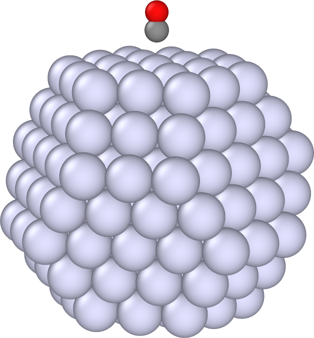
The file struct.xyz contains the structure of an Ag nanoparticle with the CO molecule adsorbed on a (111) on-top site.

We read the file and set up an ground state calculation in GPAW.

• We use LCAO mode

• We use the GLLB-sc xc-functional

The configuration options and details on how to run the calculation in parallel using MPI can be found in the GPAW documentation.

from ase.io import read
from gpaw import GPAW

atoms = read('struct.xyz')

# Add dipole moment corrections to center of metallic nanoparticle
metal_i = [sym in ['Na', 'Al', 'Ag', 'Au', 'Cu'] for sym in atoms.get_chemical_symbols()]
center = atoms.get_positions()[metal_i].mean(axis=0)
parprint(f'Center of NP is at {center}', flush=True)
moment_corrections = [dict(moms=range(1+3), center=center)]

calc_kwargs = {}
calc_kwargs['mode'] = 'lcao'  # LCAO mode
calc_kwargs['h'] = 0.2  # Grid spacing in Å
calc_kwargs['setups'] = {'Ag': '11'}
calc_kwargs['basis'] = {elem: 'pvalence.dz' for elem in ['Ag', 'Au', 'Cu']}
calc_kwargs['poissonsolver'] = {'name': 'MomentCorrectionPoissonSolver',
                                'moment_corrections': moment_corrections,
                                'poissonsolver': 'fast'}
calc_kwargs['mixer'] = {'beta': 0.1, 'nmaxold': 5, 'weight': 50.0}
calc_kwargs['symmetry'] = {'point_group': False}  # Necessary for RT-TDDFT
calc_kwargs['occupations'] = {'name': 'fermi-dirac', 'width': 0.05}
calc_kwargs['maxiter'] = 450
calc_kwargs['xc'] = 'GLLBSC'
calc_kwargs['txt'] = 'gs.out'

calc_kwargs['nbands'] = -200
calc_kwargs['convergence'] = {'density': 1e-12, 'bands': -150}

# Set up calculator and converge ground state
calc = GPAW(**calc_kwargs)
calc.get_potential_energy()

# Write the ground state to file
calc.write('gs.gpw', mode='all')

For later analysis, we will need to compute the KS wave functions in the full space, including all unoccupied states. We also construct a KohnShamDecomposition object to hold some additional information, like the dipole operator in the KS basis.

from ase.parallel import parprint
from gpaw import GPAW
from gpaw.lcaotddft.ksdecomposition import KohnShamDecomposition

gpwfile = 'gs.gpw'
gsunoccfile = 'gs_unocc.gpw'
ksdfile = 'ksd.ulm'

# Calculate ground state with full unoccupied space
parprint('Loading GS with full unoccupied space', flush=True)
parallel = {"sl_auto": True, "domain": 1, "augment_grids": True}
calc = GPAW(gpwfile, txt='/dev/stdout', parallel=parallel)
calc = calc.fixed_density(nbands='nao', convergence={'density': 1e-12}, parallel=parallel)

calc.get_potential_energy()

parprint(f'Saving GS with full unoccupied space to {gsunoccfile}', flush=True)
calc.write(gsunoccfile, mode='all')

# Construct KS electron-hole basis
ksd = KohnShamDecomposition(calc)
ksd.initialize(calc)
ksd.write(ksdfile)
parprint(f'Saving Kohn-Sham decomposition to {ksdfile}', flush=True)

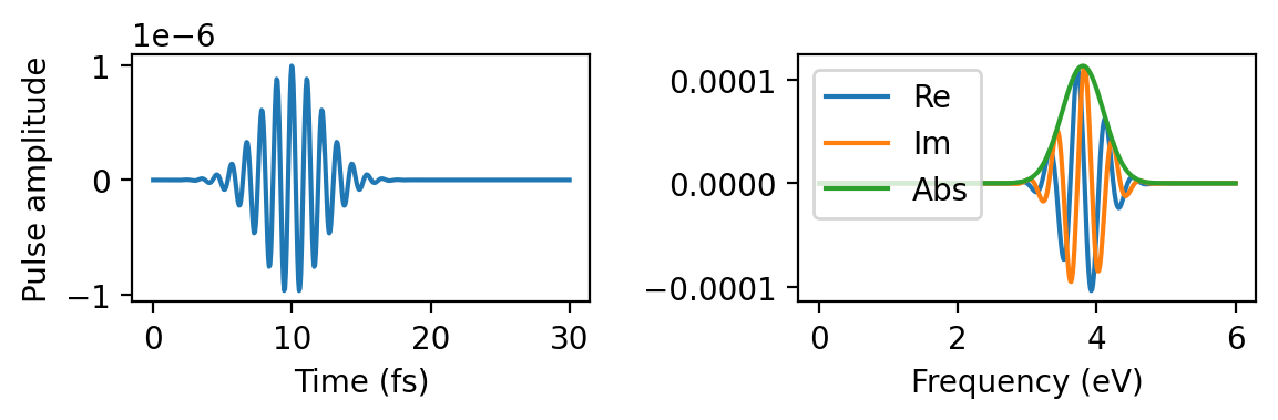
Now we load the ground state file (the first file, with only the occupied states) and perform time propagation under some external field. We choose a spatially uniform (we are in the long-wavelength limit) field with a Gaussian temporal shape.

It is instructive to first plot the pulse

import numpy as np
from gpaw.tddft.units import eV_to_au, fs_to_au, au_to_fs
from matplotlib import pyplot as plt
from gpaw.lcaotddft.laser import GaussianPulse

def create_pulse():
    strength = 1e-6  # Amplitude
    time0 = 10e3  # Time of maximum in attoseconds
    frequency = 3.8  # Frequency in eV
    sigma = 0.3  # Width parameter in eV

    # Transform the sigma parameter of the Gaussian to a full-width at half-maximum
    fwhm_eV = np.sqrt(8 * np.log(2)) * sigma
    fwhm_fs = np.sqrt(8 * np.log(2)) / (sigma * eV_to_au) * au_to_fs

    print(f'Full width at half-maximum in time {fwhm_fs:.2f}fs')
    print(f'Full width at half-maximum in frequency {fwhm_eV:.2f}eV')

    # Temporal shape of the time-dependent potential
    pulse = GaussianPulse(strength, time0, frequency, sigma, 'cos')

    return pulse

fig, axes = plt.subplots(1, 2, figsize=(6, 2), dpi=200)

time = np.linspace(0, 30, 500)  # Time grid in femtoseconds for plotting
frequency = np.linspace(0, 6, 500)  # Frequency grid in eV for plotting
pulse = create_pulse()

axes[0].plot(time, pulse.strength(time * fs_to_au))
axes[0].set_xlabel('Time (fs)')
axes[0].set_ylabel('Pulse amplitude')

axes[1].plot(frequency, pulse.fourier(frequency * eV_to_au).real, label='Re')
axes[1].plot(frequency, pulse.fourier(frequency * eV_to_au).imag, label='Im')
axes[1].plot(frequency, np.abs(pulse.fourier(frequency * eV_to_au)), label='Abs')
axes[1].set_xlabel('Frequency (eV)')
axes[1].legend(loc='upper left')

fig.tight_layout()

Full width at half-maximum in time 5.17fs
Full width at half-maximum in frequency 0.71eV

Now we perform the time propagation. This is out most time consuming task. We refer to the GPAW documentation on how to run using MPI and restart files.

• We attach a DipoleMomentWriter that writes the dipole moment at every timestep to dm_gauss.dat

• We attach a WaveFunctionWriter that writes the LCAO wave function coefficients to wfs_gauss.ulm. To save space, we write it every 10 steps

import numpy as np
from ase.units import Hartree, Bohr
from gpaw.external import ConstantElectricField
from gpaw.lcaotddft import LCAOTDDFT
from gpaw.lcaotddft.laser import GaussianPulse
from gpaw.lcaotddft.dipolemomentwriter import DipoleMomentWriter
from gpaw.lcaotddft.wfwriter import WaveFunctionWriter

# Temporal shape of the time-dependent potential
pulse = create_pulse()
# Spatial shape of the time-dependent potential
ext = ConstantElectricField(Hartree / Bohr, [0., 0., 1.])
# Time-dependent potential
td_potential = {'ext': ext, 'laser': pulse}

# Set up the time-propagation calculation
td_calc = LCAOTDDFT('gs.gpw', td_potential=td_potential, txt='td_gauss.out')

# Attach the data recording and analysis tools
DipoleMomentWriter(td_calc, 'dm_gauss.dat')
WaveFunctionWriter(td_calc, 'wfs_gauss.ulm', interval=10)

# Propagate
td_calc.propagate(20, 1500)  # 1500 steps of 20 as

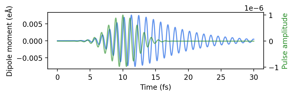
Analyzing the induced dipole moment

Let us plot the induced dipole moment by reading the dm_gauss.dat file. The system responds to the applied pulse by oscillating strongly. After the pulse has reached its maximum, however, the dipole moment of the system keeps oscillating. The amplitude of the oscillations slowly decreases over the remainder of the calculation.

from ase.units import Bohr

data = np.load('dm_gauss.npz')

time = data['time_t'] * au_to_fs  # Convert from atomic units to femtoseconds
dipmom = data['dm_tv'][:, 2] * Bohr  # Convert from atomic units to eÅ

pulse = create_pulse()

fig, ax = plt.subplots(1, 1, figsize=(6, 2), dpi=200)
twinax = ax.twinx()

twinax.plot(time, pulse.strength(time * fs_to_au), color='forestgreen', alpha=0.6)
ax.plot(time, dipmom - dipmom[0], color='cornflowerblue')

ax.set_xlabel('Time (fs)')
ax.set_ylabel('Dipole moment (eÅ)')
twinax.set_ylabel('Pulse amplitude', color='forestgreen')

fig.tight_layout()

Full width at half-maximum in time 5.17fs
Full width at half-maximum in frequency 0.71eV

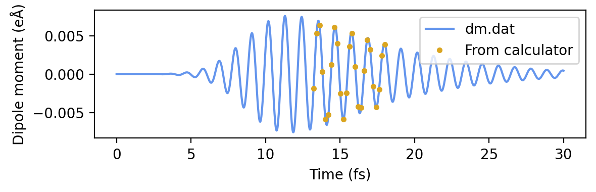
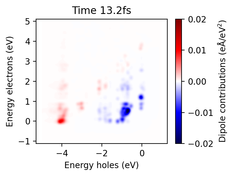
Let us analyze the system at a moment in time when the oscillations are large. The dipole moment can be expressed as

\[\boldsymbol{d}(t) = \sum_{ia} \boldsymbol{d}_{ia} \rho_{ia}(t),\]

where \(\boldsymbol{d}_{ia}\) is the dipole operator in the basis of ground state Kohn-Sham (KS) orbitals, and \(\rho_{ia}(t)\) the KS-density matrix in the basis of ground state KS orbitals. By calculating and plotting \(\boldsymbol{d}_{ia} \rho_{ia}(t)\) we can find out which the states contribute the most to the dipole moment. The dipole matrix is \(\boldsymbol{d}_{ia}\) is stored in ksd.ulm, which we have already computed.

We compute \(\rho_{ia}(t)\) using the TimeDensityMatricesFromWaveFunctions. We initialize this object with the filename of the KohnShamDecomposition file, the file name of the wave function dump file, and a list of times \(t\), in attoseconds, for which we want to compute the density matrices. The TimeDensityMatricesFromWaveFunctions will choose times that are present in the wave function dump, and that are as close as possible to the specified times. For now, we focus on \(t = 13\,\)fs.

For the purpose of visualization, we want to construct a transition contribution map where the discrete matrix elements \(\boldsymbol{d}_{ia} \rho_{ia}(t)\) are broadened onto an energy grid

\[\boldsymbol{d}(t, \varepsilon_o, \varepsilon_u) = \sum_{ia} \boldsymbol{d}_{ia} \rho_{ia}(t) G(\varepsilon_i - \varepsilon_o; \sigma) G(\varepsilon_a - \varepsilon_u; \sigma)\]

by convolution with Gaussians \(G(\varepsilon_i - \varepsilon_o; \sigma)\) of width \(\sigma\) centered on the KS eigenenergies \(\varepsilon_i\).

We use the DipoleCalculator to calculate the product \(\boldsymbol{d}_{ia} \rho_{ia}(t)\) and broaden it on the energy grid. We give the DipoleCalculator the density matrices object, energy grids \(\varepsilon_o\) and \(\varepsilon_u\) for the occupied and unoccupied energies grid, and a \(\sigma\) parameter of 0.07eV. Then we use icalculate_gather_on_root(yield_total_ou=True, v=2) to iteratively compute this quantity for each time and the \(z\) component. In general, this function is able to work in parallel across many MPI ranks, and broadcast the results to only the root rank. Since we have only specified one time, it will only yield one result. We obtain the broadened grid from res['dm_ou'] and the actual time from metadata.time.

import numpy as np
from matplotlib import pyplot as plt
from matplotlib.colors import Normalize

from rhodent.density_matrices import TimeDensityMatricesFromWaveFunctions
from rhodent.calculators.dipole import DipoleCalculator

# Set up the density matrices object
density_matrices = TimeDensityMatricesFromWaveFunctions(
    ksd='ksd.ulm',
    wfs_fname='wfs_gauss.ulm',
    times=np.arange(13100, 18000, 100))

# Set up the dipole calculator that calculates and broadens dipole contributions onto an energy grid
calc = DipoleCalculator(density_matrices, None, energies_occ=np.arange(-5, 1, 0.01), energies_unocc=np.arange(-1, 5, 0.01), sigma=0.07)

time_from_calc = density_matrices.times * 1e-3
dipmom_from_calc = []
# Iterate over the results
for metadata, res in calc.icalculate_gather_on_root(v=2):
    dipmom_from_calc.append(res['dm'])

[0000/0001] [00:00:00.0] Opened item #0
[0000/0001] [00:00:00.0] Opened item #100
[0000/0001] [00:00:00.0] Opened item #200
[0000/0001] [00:00:00.0] Opened item #300
[0000/0001] [00:00:00.1] (on 1 ranks) Constructing C0_sknM
[0000/0001] [00:00:20.9] (on 1 ranks) Constructed C0_sknM
[0000/0001] [00:00:20.9] (on 1 ranks) Constructing rho0_skMM
[0000/0001] [00:00:33.4] (on 1 ranks) Constructed rho0_skMM
[0000/0001] [00:00:39.8] Calculated and broadened dipoles contributions in 0.02s for 13110.0as
[0000/0001] [00:00:46.2] Calculated and broadened dipoles contributions in 0.02s for 13210.0as
[0000/0001] [00:00:52.6] Calculated and broadened dipoles contributions in 0.02s for 13310.0as
[0000/0001] [00:00:59.0] Calculated and broadened dipoles contributions in 0.01s for 13410.0as
[0000/0001] [00:01:05.4] Calculated and broadened dipoles contributions in 0.01s for 13510.0as
[0000/0001] [00:01:11.8] Calculated and broadened dipoles contributions in 0.02s for 13610.0as
[0000/0001] [00:01:18.2] Calculated and broadened dipoles contributions in 0.01s for 13710.0as
[0000/0001] [00:01:24.6] Calculated and broadened dipoles contributions in 0.02s for 13810.0as
[0000/0001] [00:01:31.0] Calculated and broadened dipoles contributions in 0.02s for 13910.0as
[0000/0001] [00:01:37.4] Calculated and broadened dipoles contributions in 0.01s for 14010.0as
[0000/0001] [00:01:43.8] Calculated and broadened dipoles contributions in 0.02s for 14110.0as
[0000/0001] [00:01:50.2] Calculated and broadened dipoles contributions in 0.01s for 14210.0as
[0000/0001] [00:01:56.6] Calculated and broadened dipoles contributions in 0.02s for 14310.0as
[0000/0001] [00:02:03.0] Calculated and broadened dipoles contributions in 0.01s for 14410.0as
[0000/0001] [00:02:09.4] Calculated and broadened dipoles contributions in 0.02s for 14510.0as
[0000/0001] [00:02:15.7] Calculated and broadened dipoles contributions in 0.02s for 14610.0as
[0000/0001] [00:02:22.1] Calculated and broadened dipoles contributions in 0.01s for 14710.0as
[0000/0001] [00:02:28.5] Calculated and broadened dipoles contributions in 0.02s for 14810.0as
[0000/0001] [00:02:34.9] Calculated and broadened dipoles contributions in 0.01s for 14910.0as
[0000/0001] [00:02:41.3] Calculated and broadened dipoles contributions in 0.01s for 15010.0as
[0000/0001] [00:02:47.7] Calculated and broadened dipoles contributions in 0.01s for 15110.0as
[0000/0001] [00:02:54.1] Calculated and broadened dipoles contributions in 0.02s for 15210.0as
[0000/0001] [00:03:00.5] Calculated and broadened dipoles contributions in 0.02s for 15310.0as
[0000/0001] [00:03:06.9] Calculated and broadened dipoles contributions in 0.01s for 15410.0as
[0000/0001] [00:03:13.3] Calculated and broadened dipoles contributions in 0.02s for 15510.0as
[0000/0001] [00:03:19.7] Calculated and broadened dipoles contributions in 0.01s for 15610.0as
[0000/0001] [00:03:26.1] Calculated and broadened dipoles contributions in 0.01s for 15710.0as
[0000/0001] [00:03:32.5] Calculated and broadened dipoles contributions in 0.01s for 15810.0as
[0000/0001] [00:03:38.9] Calculated and broadened dipoles contributions in 0.02s for 15910.0as
[0000/0001] [00:03:45.2] Calculated and broadened dipoles contributions in 0.02s for 16010.0as
[0000/0001] [00:03:51.6] Calculated and broadened dipoles contributions in 0.01s for 16110.0as
[0000/0001] [00:03:58.0] Calculated and broadened dipoles contributions in 0.02s for 16210.0as
[0000/0001] [00:04:04.4] Calculated and broadened dipoles contributions in 0.02s for 16310.0as
[0000/0001] [00:04:10.8] Calculated and broadened dipoles contributions in 0.02s for 16410.0as
[0000/0001] [00:04:17.2] Calculated and broadened dipoles contributions in 0.02s for 16510.0as
[0000/0001] [00:04:23.6] Calculated and broadened dipoles contributions in 0.02s for 16610.0as
[0000/0001] [00:04:30.0] Calculated and broadened dipoles contributions in 0.01s for 16710.0as
[0000/0001] [00:04:36.4] Calculated and broadened dipoles contributions in 0.01s for 16810.0as
[0000/0001] [00:04:42.8] Calculated and broadened dipoles contributions in 0.02s for 16910.0as
[0000/0001] [00:04:49.2] Calculated and broadened dipoles contributions in 0.01s for 17010.0as
[0000/0001] [00:04:55.6] Calculated and broadened dipoles contributions in 0.02s for 17110.0as
[0000/0001] [00:05:02.0] Calculated and broadened dipoles contributions in 0.01s for 17210.0as
[0000/0001] [00:05:08.4] Calculated and broadened dipoles contributions in 0.01s for 17310.0as
[0000/0001] [00:05:14.8] Calculated and broadened dipoles contributions in 0.01s for 17410.0as
[0000/0001] [00:05:21.2] Calculated and broadened dipoles contributions in 0.02s for 17510.0as
[0000/0001] [00:05:27.6] Calculated and broadened dipoles contributions in 0.01s for 17610.0as
[0000/0001] [00:05:34.0] Calculated and broadened dipoles contributions in 0.01s for 17710.0as
[0000/0001] [00:05:40.4] Calculated and broadened dipoles contributions in 0.02s for 17810.0as
[0000/0001] [00:05:46.8] Calculated and broadened dipoles contributions in 0.01s for 17910.0as
[0000/0001] [00:05:46.8] Finished calculating dipoles contributions

# Plot the dipole moment and the dipole moment contributions
fig, ax = plt.subplots(1, 1, figsize=(6, 2), dpi=200)
ax.set_xlabel('Time (fs)')
ax.set_ylabel('Dipole moment (eÅ)')

ax.plot(time, dipmom - dipmom[0], color='cornflowerblue', label='dm.dat')
ax.plot(time_from_calc, np.array(dipmom_from_calc), '.', color='goldenrod', label='From calculator')
ax.legend()

fig.tight_layout()

# Get only the first result without recreating the TimeDensityMatrices object
for metadata, res in calc.icalculate_gather_on_root(yield_total_ou=True, v=2):
    tcm = res['dm_ou']
    break

[0000/0001] [00:05:57.0] Calculated and broadened dipoles contributions in 3.57s for 13110.0as

# Plot the dipole moment and the dipole moment contributions
fig, ax = plt.subplots(1, 1, figsize=(4, 3), dpi=200)

p = ax.pcolormesh(calc.energies_occ, calc.energies_unocc, tcm.T, cmap='seismic', norm=Normalize(-0.02, 0.02))
ax.set_title(f'Time {metadata.time*1e-3:.1f}fs')
ax.axis('equal')
fig.colorbar(p, ax=ax, label='Dipole contributions (eÅ/eV$^2$)')


ax.set_ylabel('Energy electrons (eV)')
ax.set_xlabel('Energy holes (eV)')

fig.tight_layout()

The calculation of density matrices takes some time, even if it is orders of magnitudes faster than the time propagation. It is useful to perform the calculation and write the results to a file. This is done using the calculate_and_save_ulm function. The ULM file format is useful for writing large matrices without having to store them entirely in memory.

import numpy as np

from rhodent.density_matrices import TimeDensityMatricesFromWaveFunctions
from rhodent.writers.tcm import calculate_and_save_ulm

# Set up the density matrices object
density_matrices = TimeDensityMatricesFromWaveFunctions(
    ksd='ksd.ulm',
    wfs_fname='wfs_gauss.ulm',
    times=[6200])

# Calculate the transition contribution map and save it to a file
calculate_and_save_ulm('tcm_gauss.ulm', density_matrices, None, energies_occ=np.arange(-5, 1, 0.01), energies_unocc=np.arange(-1, 5, 0.01), sigma=0.07)

[0000/0001] [00:00:00.0] Opened item #0
[0000/0001] [00:00:00.0] Opened item #100
[0000/0001] [00:00:00.0] Opened item #200
[0000/0001] [00:00:00.0] Opened item #300
[0000/0001] [00:00:00.1] Will use 0.0MiB per rank (total 0.0 GiB on 1 ranks)
[0000/0001] [00:00:00.1] (on 1 ranks) Constructing C0_sknM
[0000/0001] [00:00:20.9] (on 1 ranks) Constructed C0_sknM
[0000/0001] [00:00:20.9] (on 1 ranks) Constructing rho0_skMM
[0000/0001] [00:00:33.4] (on 1 ranks) Constructed rho0_skMM
[0000/0001] [00:00:39.9] Calculated and broadened dipoles contributions in 0.01s for 6210.0as
[0000/0001] [00:00:39.9] Finished calculating dipoles contributions
Written tcm_gauss.ulm

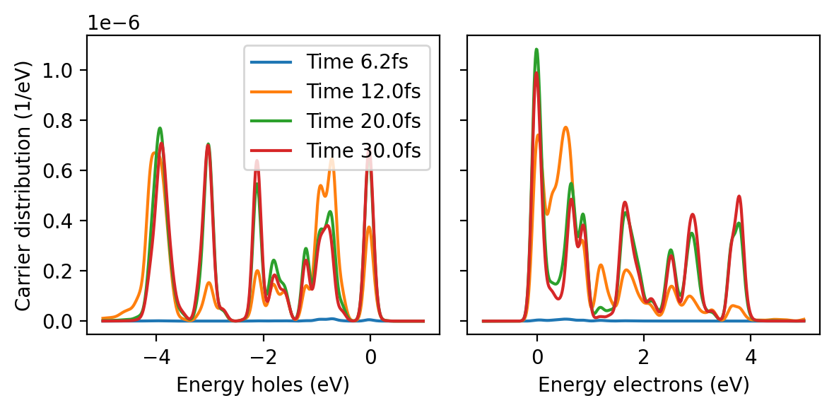
Analyzing the hot-carrier populations

The diagonals of the KS density matrix can be interpreted as the population of ground state KS orbitals. We use the calculate_hcdist_and_save_by_filename to calculate these and save to a file that we later plot.

By using a file name with the ‘.dat’ extension, it is formatted as a space-separated text file. Alternatively, you can provide the ‘.npz’ extension to save as a numpy archive.

from rhodent.density_matrices import TimeDensityMatricesFromWaveFunctions
from rhodent.writers.hcdist import calculate_hcdist_and_save_by_filename

# Set up the density matrices object
density_matrices = TimeDensityMatricesFromWaveFunctions(
    ksd='ksd.ulm',
    wfs_fname='wfs_gauss.ulm',
    times=[6200, 12000, 20000, 30000])

# Calculate the hot carrier distributions and save them to a file
calculate_hcdist_and_save_by_filename('hcdist_gauss.dat', density_matrices=density_matrices, voronoi=None, energies_occ=np.arange(-5, 1, 0.01), energies_unocc=np.arange(-1, 5, 0.01), sigma=0.07, average_times=False)

[0000/0001] [00:00:00.0] Opened item #0
[0000/0001] [00:00:00.0] Opened item #100
[0000/0001] [00:00:00.0] Opened item #200
[0000/0001] [00:00:00.0] Opened item #300
[0000/0001] [00:00:00.1] Will use 0.0MiB per rank (total 0.0GiB on 1 ranks)
[0000/0001] [00:00:00.1] (on 1 ranks) Constructing C0_sknM
[0000/0001] [00:00:20.9] (on 1 ranks) Constructed C0_sknM
[0000/0001] [00:00:20.9] (on 1 ranks) Constructing rho0_skMM
[0000/0001] [00:00:33.3] (on 1 ranks) Constructed rho0_skMM
[0000/0001] [00:00:40.1] Calculated and broadened HC distributions in 40.08s for 6210.0as
[0000/0001] [00:00:47.0] Calculated and broadened HC distributions in 46.95s for 12010.0as
[0000/0001] [00:00:53.8] Calculated and broadened HC distributions in 53.80s for 20010.0as
[0000/0001] [00:01:00.6] Calculated and broadened HC distributions in 60.61s for 30010.0as
[0000/0001] [00:01:00.6] Finished calculating hot-carrier matrices
Written hcdist_gauss.dat

!head hcdist_gauss.dat

# Hot carrier (H=hole, E=electron) distributions relative to Fermi level
# Computed for the following 4 times (in fs)
#   6.2100
#   12.0100
#   20.0100
#   30.0100
# Gaussian folding, Width 0.0700eV
# H energy (eV)   E energy (eV)     Total H (1/eV)     Total E (1/eV)  ... repeated for next times
      -5.000000       -1.000000     4.35715498e-11     1.89845675e-46     1.60970232e-08     1.50988580e-43     3.10678736e-09     3.32019067e-43     6.36711809e-10     3.14757184e-43
      -4.990000       -0.990000     4.42216133e-11     1.17756083e-45     1.62543482e-08     9.35920736e-43     3.15439518e-09     2.05757663e-42     6.48529095e-10     1.95064822e-42

from matplotlib import pyplot as plt

fig, axes = plt.subplots(1, 2, sharey=True, figsize=(6, 3), dpi=200)

data = np.loadtxt('hcdist_gauss.dat')
energies_occ = data[:, 0]
energies_unocc = data[:, 1]

times = [6.21, 12.01, 20.01, 30.01]
for t, time in enumerate(times):
    hcdist_o = data[:, 2 + 2 * t]
    hcdist_u = data[:, 3 + 2 * t]
    axes[0].plot(energies_occ, hcdist_o, label=f'Time {time:.1f}fs')
    axes[1].plot(energies_unocc, hcdist_u)

axes[0].set_ylabel('Carrier distribution (1/eV)')
axes[0].set_xlabel('Energy holes (eV)')
axes[1].set_xlabel('Energy electrons (eV)')
axes[0].legend()

fig.tight_layout()

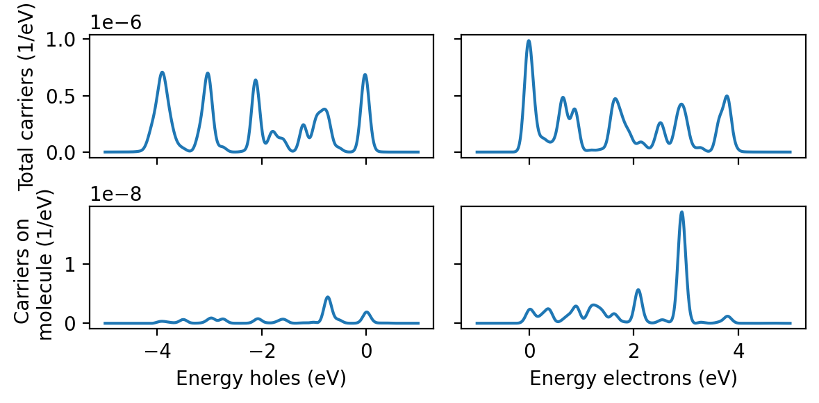
Where are the hot carriers localized?

Since we have the density matrix, we can decompose it by any means we want. The calculators support projection on ground state KS states according to a Voronoi weight. This weight is defined

\[w_{nn'} = \int_\text{partition} \psi_n(\boldsymbol{r})\psi_{n'}(\boldsymbol{r})\mathrm{d}\boldsymbol{r},\]

where the intergral is taken in the Voronoi partition of one or several atoms in space.

Compute the Voronoi decomposition of weights on the carbon and oxygen atoms, which are numbered 201 and 202, using the VoronoiWeightCalculator and VoronoiLCAOWeightCalculator. Save the decomposition to a file voronoi.ulm using calculate_and_save_by_filename. Then we load the voronoi weights using the VoronoiReader and pass it to the calculate_hcdist_and_save_by_filename function.

Alternatively, it is also possible to calculate the weights on the fly by passing the VoronoiWeightCalculator directly to the calculator.

from rhodent.voronoi import VoronoiWeightCalculator, VoronoiLCAOWeightCalculator
from rhodent.writers.voronoi import calculate_and_save_by_filename

voronoi_lcao = VoronoiLCAOWeightCalculator([[201, 202]], 'gs_unocc.gpw', domain=1, use_pblas=True)
voronoi = VoronoiWeightCalculator(voronoi_lcao, use_pblas=True)

calculate_and_save_by_filename('voronoi.ulm', voronoi=voronoi)

[0000/0001] [00:00:00.0] Start
[0000/0001] [00:00:32.6] compute a_g
[0000/0001] [00:02:41.7] Computed Voronoi decomposition grid
[0000/0001] [00:02:41.7] Start
[0000/0001] [00:03:35.4] Computed LCAO weights for projection [201, 202]
[0000/0001] [00:03:35.4] Gather P_ani
[0000/0001] [00:03:35.4] Done gathering
[0000/0001] [00:03:35.4] Distribute C_nM and P_ani
[0000/0001] [00:03:35.5] Done distributing
[0000/0001] [00:03:35.5] Distributed vt_MM
[0000/0001] [00:03:38.4] Calculated vt_nn in parallel
[0000/0001] [00:03:38.4] Distributed vt_nn
[0000/0001] [00:03:38.5] Calculated correction
Written voronoi.ulm

from rhodent.density_matrices import TimeDensityMatricesFromWaveFunctions
from rhodent.voronoi import VoronoiReader
from rhodent.writers.hcdist import calculate_hcdist_and_save_by_filename

# Set up the density matrices object
density_matrices = TimeDensityMatricesFromWaveFunctions(
    ksd='ksd.ulm',
    wfs_fname='wfs_gauss.ulm',
    times=[30000])

# Set up the Voronoi file reader
voronoi = VoronoiReader('voronoi.ulm')

# Calculate the hot carrier distributions and save them to a file
calculate_hcdist_and_save_by_filename('hcdist_gauss_proj.dat', density_matrices=density_matrices, voronoi=voronoi, energies_occ=np.arange(-5, 1, 0.01), energies_unocc=np.arange(-1, 5, 0.01), sigma=0.07, average_times=False)

[0000/0001] [00:00:00.0] Opened item #0
[0000/0001] [00:00:00.0] Opened item #100
[0000/0001] [00:00:00.0] Opened item #200
[0000/0001] [00:00:00.0] Opened item #300
[0000/0001] [00:00:00.1] Will use 0.0MiB per rank (total 0.0GiB on 1 ranks)
[0000/0001] [00:00:00.2] (on 1 ranks) Constructing C0_sknM
[0000/0001] [00:00:20.9] (on 1 ranks) Constructed C0_sknM
[0000/0001] [00:00:20.9] (on 1 ranks) Constructing rho0_skMM
[0000/0001] [00:00:33.4] (on 1 ranks) Constructed rho0_skMM
[0000/0001] [00:00:40.2] Calculated and broadened HC distributions in 40.23s for 30010.0as
[0000/0001] [00:00:40.2] Finished calculating hot-carrier matrices
Written hcdist_gauss_proj.dat

!head hcdist_proj.dat

# Hot carrier (H=hole, E=electron) distributions relative to Fermi level
# Computed for the following 1 times (in fs)
#   30.0100
# Atomic projections
#      0: [201, 202]
# Gaussian folding, Width 0.0700eV
# H energy (eV)   E energy (eV)   Total H (1/eV)     Total E (1/eV)     Proj H  0 (1/eV) Proj E  0 (1/eV) ... repeated for next times
      -5.000000       -1.000000     2.43832183e-09     1.88663412e-45     2.01350729e-12     1.45567071e-48
      -4.990000       -0.990000     2.46605230e-09     1.16934781e-44     1.99783834e-12     9.04610658e-48
      -4.980000       -0.980000     2.49902568e-09     7.10139363e-44     1.98207627e-12     5.50866655e-47

from matplotlib import pyplot as plt

data = np.loadtxt('hcdist_gauss_proj.dat')

energies_occ = data[:, 0]
energies_unocc = data[:, 1]

fig, axes = plt.subplots(2, 2, sharey='row', sharex='col', figsize=(6, 3), dpi=200)

axes[0, 0].plot(energies_occ, data[:, 2])
axes[0, 1].plot(energies_unocc, data[:, 3])
axes[1, 0].plot(energies_occ, data[:, 4])
axes[1, 1].plot(energies_unocc, data[:, 5])

axes[0, 0].set_ylabel('Total carriers (1/eV)')
axes[1, 0].set_ylabel('Carriers on \n molecule (1/eV)')
axes[-1, 0].set_xlabel('Energy holes (eV)')
axes[-1, 1].set_xlabel('Energy electrons (eV)')

fig.tight_layout()

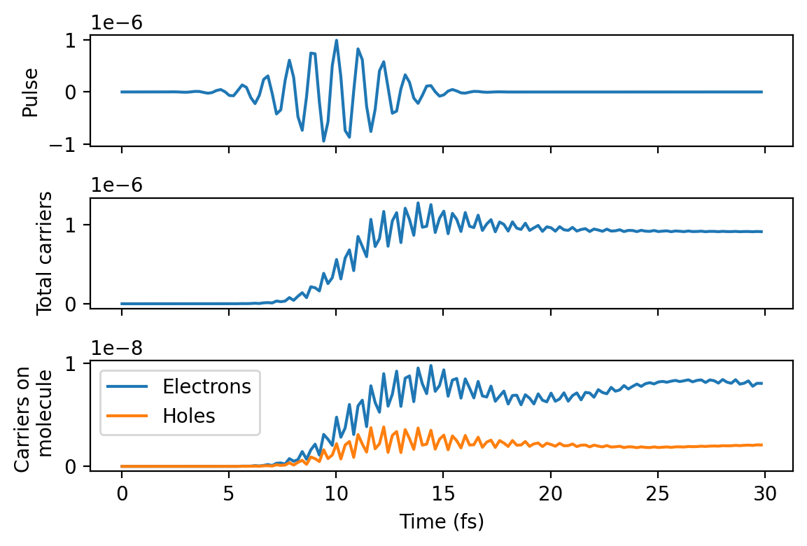
Obtaining the total number of carriers

If we are not interested in hot-carrier distributions, but only the total number of generated carriers in the respective regions, then we can use the calculate_hcsweeptime_and_save_by_filename writer instead.

import numpy as np
from gpaw.lcaotddft.laser import GaussianPulse
from rhodent.density_matrices import TimeDensityMatricesFromWaveFunctions
from rhodent.voronoi import VoronoiReader
from rhodent.writers.hcdist import calculate_hcsweeptime_and_save_by_filename

# Set up the density matrices object
density_matrices = TimeDensityMatricesFromWaveFunctions(
    ksd='ksd.ulm',
    wfs_fname='wfs_gauss.ulm',
    times=np.arange(0, 30e3, 100))

# Set up the Voronoi file reader
voronoi = VoronoiReader('voronoi.ulm')

# Calculate the hot carrier distributions and save them to a file
calculate_hcsweeptime_and_save_by_filename('hcdist_gauss_time.dat', density_matrices=density_matrices, voronoi=voronoi)

!head hcdist_gauss_time.dat

# Hot carrier (H=hole, E=electron) numbers
#
# Atomic projections:
#      0: [201, 202]
#
#       Time (fs)         Total H         Total E       Proj H  0       Proj E  0
         0.010000  1.74890287e-20  1.74890287e-20  1.90934760e-22  2.82953480e-22
         0.110000  3.65596345e-18  3.65596345e-18  3.21160307e-20  6.43713037e-20
         0.210000  1.36184834e-17  1.36184834e-17  1.10310503e-19  2.58821552e-19
         0.310000  1.96907207e-17  1.96907207e-17  1.40509699e-19  4.03688628e-19

import numpy as np
from matplotlib import pyplot as plt

data = np.loadtxt('hcdist_gauss_time.dat')

time = data[:, 0]

fig, axes = plt.subplots(3, 1, sharey='row', sharex='col', figsize=(6, 4), dpi=200)

axes[0].plot(time, pulse.strength(time * fs_to_au))
axes[1].plot(time, data[:, 2])
axes[2].plot(time, data[:, 4], label='Electrons')
axes[2].plot(time, data[:, 3], label='Holes')

axes[0].set_ylabel('Pulse')
axes[1].set_ylabel('Total carriers')
axes[2].set_ylabel('Carriers on \n molecule')
axes[2].legend()
axes[-1].set_xlabel('Time (fs)')

fig.tight_layout()

References

Kuisma, A. Sakko, T. P. Rossi, A. H. Larsen, J. Enkovaara, L. Lehtovaara, and T. T. Rantala, Localized surface plasmon resonance in silver nanoparticles: Atomistic first-principles time-dependent density-functional theory calculations, Phys. Rev. B 91, 115431 (2015).